IEOR 290A – L 12 P L M 1 Model
advertisement
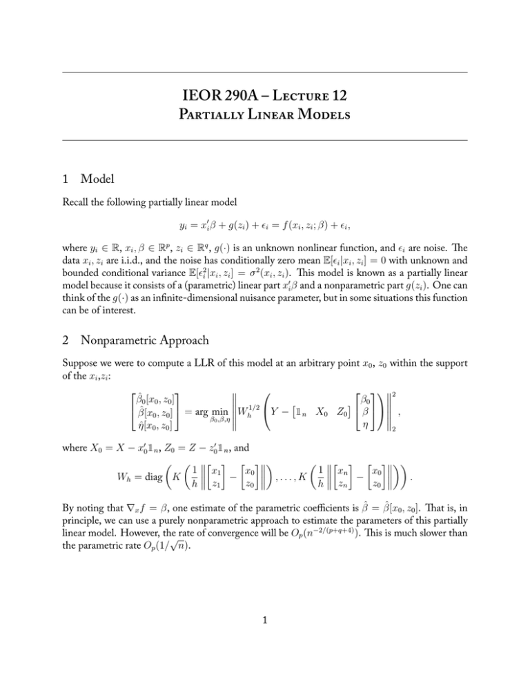
IEOR 290A – L 12 P L M 1 Model Recall the following partially linear model yi = x′i β + g(zi ) + ϵi = f (xi , zi ; β) + ϵi , where yi ∈ R, xi , β ∈ Rp , zi ∈ Rq , g(·) is an unknown nonlinear function, and ϵi are noise. e data xi , zi are i.i.d., and the noise has conditionally zero mean E[ϵi |xi , zi ] = 0 with unknown and bounded conditional variance E[ϵ2i |xi , zi ] = σ 2 (xi , zi ). is model is known as a partially linear model because it consists of a (parametric) linear part x′i β and a nonparametric part g(zi ). One can think of the g(·) as an infinite-dimensional nuisance parameter, but in some situations this function can be of interest. 2 Nonparametric Approach Suppose we were to compute a LLR of this model at an arbitrary point x0 , z0 within the support of the xi ,zi : 2 β̂0 [x0 , z0 ] 1/2 [ ] β0 β̂[x0 , z0 ] = arg min Wh Y − 1n X0 Z0 β , β0 ,β,η η η̂[x0 , z0 ] 2 where X0 = X − x′0 1n , Z0 = Z − z0′ 1n , and ( ( [ ] [ ]) ( [ ] [ ])) 1 1 x1 x0 xn − x0 Wh = diag K − ,...,K . z0 z0 h z1 h zn By noting that ∇x f = β, one estimate of the parametric coefficients is β̂ = β̂[x0 , z0 ]. at is, in principle, we can use a purely nonparametric approach to estimate the parameters of this partially −2/(p+q+4) linear model. However, the ). is is much slower than √ rate of convergence will be Op (n the parametric rate Op (1/ n). 1 3 Semiparametric Approach √ Ideally, our estimates of β should converge at the parametric rate Op (1/ n), but the g(zi ) term causes difficulties in being able to achieve this. But if we could somehow subtract out this term, then we would be able to estimate β at the parametric rate. is is the intuition behind the semiparametric approach. Observe that E[yi |zi ] = E[x′i β + g(zi ) + ϵi |zi ] = E[xi |zi ]′ β + g(zi ), and so yi − E[yi |zi ] = (x′i β + g(zi ) + ϵi ) − E[xi |zi ]′ β − g(zi ) = (xi − E[xi |zi ])′ β + ϵi . Now if we define E[y1 |z1 ] .. Ŷ = . E[yn |zn ] E[x1 |z1 ]′ .. X̂ = . ′ E[xn |zn ] and then we can define an estimator β̂ = arg min ∥(Y − Ŷ ) − (X − X̂)β∥22 = ((X − X̂)′ (X − X̂))−1 ((X − X̂)′ (Y − Ŷ )). β e only question is how can we compute E[xi |zi ] and E[yi |zi ]? It turns out that if we compute those values with the trimmed version of the Nadaraya-Watson estimator, then the estimate β̂ converges at the parametric rate under reasonable technical conditions. Intuitively, we would expect that we could alternatively use the L2-regularized Nadaraya-Watson estimator, but this has not yet been proven to be the case. 2
