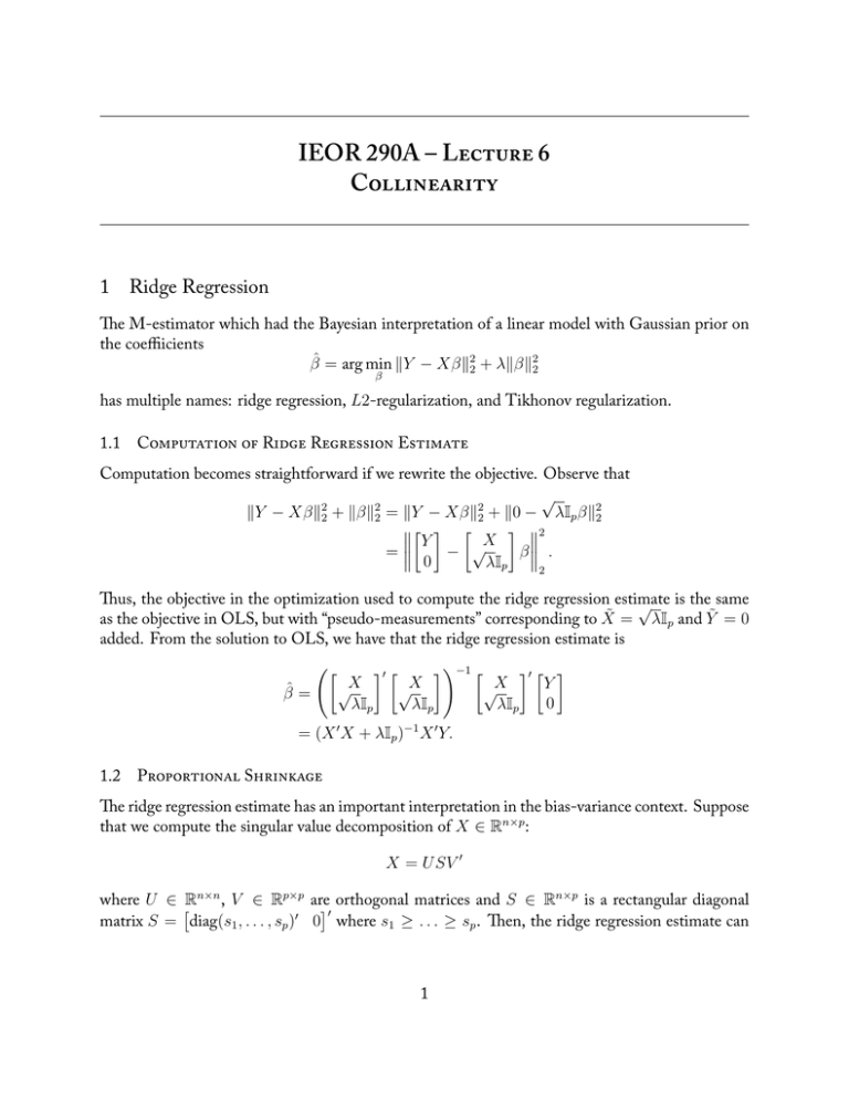
IEOR 290A – L 6
C
1
Ridge Regression
e M-estimator which had the Bayesian interpretation of a linear model with Gaussian prior on
the coeffiicients
β̂ = arg min ∥Y − Xβ∥22 + λ∥β∥22
β
has multiple names: ridge regression, L2-regularization, and Tikhonov regularization.
1.1
C  R R E
Computation becomes straightforward if we rewrite the objective. Observe that
√
∥Y − Xβ∥22 + ∥β∥22 = ∥Y − Xβ∥22 + ∥0 − λIp β∥22
[ ] [
] 2
Y
X
√
=
−
β
.
0
λIp 2
us, the objective in the optimization used to compute the ridge regression estimate
√ is the same
as the objective in OLS, but with “pseudo-measurements” corresponding to X̃ = λIp and Ỹ = 0
added. From the solution to OLS, we have that the ridge regression estimate is
([
β̂ =
√X
λIp
]′ [
√X
λIp
])−1 [
√X
λIp
]′ [ ]
Y
0
= (X ′ X + λIp )−1 X ′ Y.
1.2
P S
e ridge regression estimate has an important interpretation in the bias-variance context. Suppose
that we compute the singular value decomposition of X ∈ Rn×p :
X = U SV ′
where U ∈ Rn×n , V ∈ Rp×p are orthogonal matrices and S ∈ Rn×p is a rectangular diagonal
[
]′
matrix S = diag(s1 , . . . , sp )′ 0 where s1 ≥ . . . ≥ sp . en, the ridge regression estimate can
1
be rewritten as
β̂ = (X ′ X + λIp )−1 X ′ Y
= (V S ′ U ′ U SV ′ + λIp )−1 V S ′ U ′ Y
= (V diag(s21 , . . . , s2p )V ′ + λV V ′ )−1 V S ′ U ′ Y
)
(
1
1
,..., 2
V ′V S ′U ′Y
= V diag 2
s1 + λ
sp + λ
[
(
) ]
sp
s1
= V diag s2 +λ , . . . , s2 +λ
0 U ′ Y.
p
1
If λ = 0, then the estimate is just the OLS estimate. So one interpretation of the ridge regression
estimate is that we are shrinking the inverse of the singular values towards zero. e shrinkage is
proportional to the magnitude of si , meaning that the shrinkage is relatively smaller for si versus
si+1 .
2
Collinearity
e usage of SVD suggests a geometric interpretation may be valuable. Consider the standard
linear model yi = x′i β + ϵi , and further suppose that xi = zi′ B + µi , where zi ∈ Rd is a vector
of “hidden” variables, d < p, B ∈ Rp×d is a matrix of coefficients, and µi is zero mean noise with
finite variance. e idea of this model is that we observe xi , but xi has smaller dimensionality due
to these variables actually being an unknown function of zi that are not measured. We will assume
that zi are Gaussian and have zero mean with finite variance. For notational convenience, we define
Z ∈ Rn×d to be the matrix whose i-th row is zi′ ; similarly, we define M ∈ Rn×p to be the matrix
whose i-th row is µ′i . Lastly, we define Σ to be the covariance matrix of X, Σz to be the covariance
matrix of zi , and σ 2 I to be the covariance matrix of µi .
To understand why this situation is problematic, consider the sample covariance matrix
1
X ′X
n
p
= n1 B ′ Z ′ ZB + n1 M ′ M → Σ = B ′ Σz B + σ 2 I.
Now note that Σz has rank p, and B ′ Σz B is positive semidefinite and so can be diagonalized.
Specifically, we can write
Σ = B ′ Σz B + σ 2 I
= U diag(s1 , . . . , sd , 0, . . . , 0)U ′ + σ 2 I
= U diag(s1 + σ 2 , . . . , sd + σ 2 , σ 2 , . . . , σ 2 )U ′ .
is is a problem for two reasons. First, the small σ 2 looks like signal, but it is actually noise. Second, the small σ 2 distorts our signal (though we cannot fix this issue without specifically considering
errors-in-variables estimators).
e ridge regression estimate tries to shrink the σ 2 noise terms towards zero, while impacting
the signal terms si less (i.e., proportional shrinkage). And so ridge regression can be interpreted
in this geometrical context as trying to estimate the linear coefficients subject to a model in which
the measured variables xi as actually linear functions of a lower dimensional variable zi that is not
measured.
2
3
Exterior Derivative Estimator
Consider the collinearity model described above, and suppose that instead we only shrink the values
that we believe are noise sd+1 , . . . , sp . en we can define another estimator as
(
) ]
[
s
sp
0 U ′ Y.
β̂ = V diag s11 , . . . , s1d , s2 d+1+λ , . . . , s2 +λ
d+1
p
is estimator provides a different bias-variance tradeoff. It turns out that we can define this as the
following M-estimator
β̂ = arg min ∥Y − Xβ∥22 + λ∥Πβ∥22 ,
β
where Π is a projection matrix that projects onto the (p − d) smallest eigenvectors of the sample
covariance matrix n1 X ′ X. We call this the exterior derivative estimator (EDE).
e name for this estimator is inspired by the following question: If we estimate the β coefficients in our model, then what is their interpretation? is question looks simple, but it is more
complex than it seems at first glance. e coefficients β cannot be interpreted as a gradient because
the xi do not span the whole space. It turns out that the correct interpretation of the β in this model
is that of an exterior derivative, which is an extension of gradients to differentiable manifolds. e
intuition is that the β only gives derivative information in the directions of the manifold, but we
do not get derivative information in other directions. is is important because if we interpret,
say ridge regression, in a geometric context then it means that we have only been able to estimate
derivative information in some “measured” directions. e EDE estimate makes this intuition clear
because we are penalizing for deviations of our estimate from the “measured” directions.
3.1
P C R
ere is another regression method known as principal component regression (PCR) in which the
estimate is
[
(
) ]
1
1
β̂ = V diag s1 , . . . , sd , 0, . . . , 0 0 U ′ Y.
e normal way for writing this estimate is as a change of coordinates that converts xi into some
scaled variables in a lower dimension z̃i , builds a linear model with inputs z̃i and output yi , and
then performs the inverse coordinate change to get the linear model in the xi space. We can also
interpret PCR as a special case of the EDE. is can be seen by defining the PCR estimate as
β̂ = arg min lim ∥Y − Xβ∥22 + λ∥Πβ∥22
β
λ→∞
= lim arg min ∥Y − Xβ∥22 + λ∥Πβ∥22 .
λ→∞
β
Note that swapping the limit and minimization is not allowed in every situation, but it is allowed
in this situation. e reasons for this are technical and will be discussed later in the course.
3