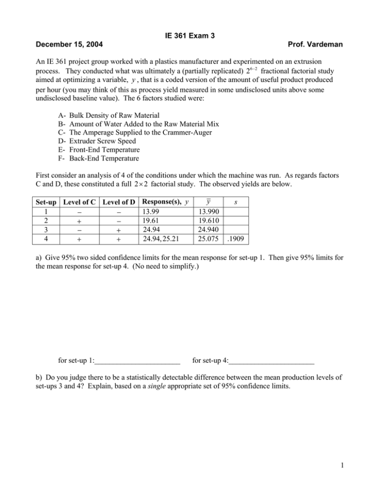
IE 361 Exam 3
December 15, 2004
Prof. Vardeman
An IE 361 project group worked with a plastics manufacturer and experimented on an extrusion
process. They conducted what was ultimately a (partially replicated) 26 − 2 fractional factorial study
aimed at optimizing a variable, y , that is a coded version of the amount of useful product produced
per hour (you may think of this as process yield measured in some undisclosed units above some
undisclosed baseline value). The 6 factors studied were:
ABCDEF-
Bulk Density of Raw Material
Amount of Water Added to the Raw Material Mix
The Amperage Supplied to the Crammer-Auger
Extruder Screw Speed
Front-End Temperature
Back-End Temperature
First consider an analysis of 4 of the conditions under which the machine was run. As regards factors
C and D, these constituted a full 2 × 2 factorial study. The observed yields are below.
Set-up Level of C Level of D Response(s), y
13.99
1
−
−
19.61
2
+
−
24.94
3
−
+
4
24.94, 25.21
+
+
y
13.990
19.610
24.940
25.075
s
.1909
a) Give 95% two sided confidence limits for the mean response for set-up 1. Then give 95% limits for
the mean response for set-up 4. (No need to simplify.)
for set-up 1:_______________________
for set-up 4:_______________________
b) Do you judge there to be a statistically detectable difference between the mean production levels of
set-ups 3 and 4? Explain, based on a single appropriate set of 95% confidence limits.
1
c) Treat the 4 set-ups listed in the table on page 1 as a 22 factorial in factors C and D. Find fitted
main effects of C and D ( c2 and d 2 ) and the fitted CD interaction ( cd 22 ) if one takes this point of view.
d) Which (if any) of the fitted/estimated effects you computed in part c) are "statistically significant"?
(Base your answer on appropriate 95% confidence limits and explain.)
e) As a matter of fact, while levels of factors A,B, and E were held constant across set-ups 1 through
4 in listed in the table on page 1, set-ups 1 and 3 were made with the high ( + ) level of factor F and setups 2 and 4 were made with the low level ( − ) of factor F. Even limiting attention to the single set of
levels of A,B and E represented in set-ups 1 through 4, this last fact (about factor F) should probably
change your interpretation of the results of parts c) and d). Explain.
We will henceforth consider the whole 26 − 2 experiment run by the students. As a matter of fact, they
used the two generators
E ↔ AB and F ↔ AC
f) What levels of E and F were used with the following combinations of A,B,C and D? (Fill in the
blanks.)
Level of A
+
+
+
Level of B
+
+
−
Level of C
+
−
−
Level of D
−
−
−
Level of E
Level of F
2
The students reported a "4 degree of freedom" pooled sample standard deviation of .37. Further, the
sum of the reciprocals of their 16 sample sizes was 14.
g) A "fitted sum of effects" computed via the Yates algorithm based on the 16 sample means can be
used to make 95% confidence limits of the form
n
fitted sum of effects ± ∆
for an appropriate value ∆ . Find this value.
Below is a table of 16 ABCDEF combinations with corresponding sample means, and a final column
that comes from use of the Yates algorithm on the sample means.
Combination
ef
a
bf
abe
ce
acf
bc
abcef
def
ad
bdf
abde
cde
acdf
bcd
abcdef
y
13.99
6.76
20.71
11.12
19.61
15.73
23.45
20.00
24.94
24.53
24.97
24.29
25.08
24.40
30.00
33.08
Output of the
Yates Algorithm
21.42
-1.43
2.04
.10
2.50
.81
.68
.43
4.99
1.59
-.36
.34
-.77
-.37
1.05
.08
h) How many "cycles" of additions and subtractions and what final divisor were used to produce the
last column in the above table?
number of cycles ____________________
final divisor ______________________
i) Circle values in the last column of the table that represent "statistically detectable sums" according
to the criterion of part g).
3
As it turns out, the pooled sample standard deviation reported by the students is probably "too small"
because their "replication" consisted of consecutive runs of the machine for a given set-up. Experience
with the machine strongly suggested that for a given combination of levels of the factors A through F,
consecutive runs for a given set-up were more homogeneous than were runs where the same
combination of levels of A through F was used, but other (different) set-ups intervened between the
runs. So the practical implications of part i) are suspect, and a second way of judging the statistical
detectability of sums of effects was tried. A normal plot of the last 15 entries in the "Output of the
Yates Algorithm" column in the table on the previous page was made. It is below.
j) On the basis of the plot above, what value(s) in the table on page 3 clearly represent statistically
detectable sum(s) of effects? Explain.
k) What is the simplest possible interpretation of your answer to j)? If the object of running the
machine is "large y " what does j) suggest about how the machine should be set up (which levels of
which factors should be used)?
l) Say why, in retrospect, your answer to k) is clearly consistent with the list of sample means in the
table on page 3.
4