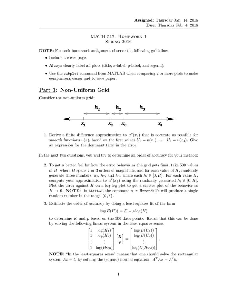
Assigned: Thursday Jan. 14, 2016
Due: Thursday Feb. 4, 2016
MATH 517: Homework 1
Spring 2016
NOTE: For each homework assignment observe the following guidelines:
• Include a cover page.
• Always clearly label all plots (title, x-label, y-label, and legend).
• Use the subplot command from MATLAB when comparing 2 or more plots to make
comparisons easier and to save paper.
Part 1: Non-Uniform Grid
Consider the non-uniform grid:
1. Derive a finite difference approximation to u00 (x2 ) that is accurate as possible for
smooth functions u(x), based on the four values U1 = u(x1 ), . . . , U4 = u(x4 ). Give
an expression for the dominant term in the error.
In the next two questions, you will try to determine an order of accuracy for your method:
2. To get a better feel for how the error behaves as the grid gets finer, take 500 values
of H, where H spans 2 or 3 orders of magnitude, and for each value of H, randomly
generate three numbers, h1 , h2 , and h3 , where each hi ∈ [0, H]. For each value H,
compute your approximation to u00 (x2 ) using the randomly generated hi ∈ [0, H].
Plot the error against H on a log-log plot to get a scatter plot of the behavior as
H → 0. NOTE: in matlab the command x = H*rand(1) will produce a single
random number in the range [0,H].
3. Estimate the order of accuracy by doing a least squares fit of the form
log(E(H)) = K + p log(H)
to determine K and p based on the 500 data points. Recall that this can be done
by solving the following linear system in the least squares sense:




1 log(H1 )
log(E(H1 ))
1 log(H2 )   log(E(H2 )) 


 K

=

.
 ..
..
..
p



.
.
.
log(E(H500 ))
1 log(H500 )
NOTE: “In the least-squares sense” means that one should solve the rectangular
system Ax = b, by solving the (square) normal equation: AT Ax = AT b.
1
Assigned: Thursday Jan. 14, 2016
Due: Thursday Feb. 4, 2016
Part 2: Mixed Conditions
Consider the following 2-point BVP:
u00 + u = f (x),
on
0
0 ≤ x ≤ 10
0
u (0) − u(0) = 0,
u (10) + u(10) = 0.
4. Construct a second-order accurate finite-difference method for this BVP. Write your
method as a linear system of the form A~u = f~.
5. Construct the exact solution to this BVP with f (x) = −ex .
6. Verify that your method is second order accurate by solving the BVP with f (x) =
−ex at four different grid spacings h.
HINT 1: Use the spdiags command in matlab to create the sparse matrix A –
this will save storage and allow matlab to use a fast solver. Modify the following
commands, which generate a tri-diagonal matrix with a [1,-2,1] structure, to model
your specific BVP:
e = ones(n,1);
A = spdiags([e -2*e e], -1:1, n, n);
HINT 2: Use the command u = A\f to invert your system – this will use a fast
solver if you created your matrix with spdiags.
Part 3: Periodic Boundary Conditions
Consider the following 2-point BVP:
−u00 + u = f (x),
0
on
0
u(0) = u(1) u (0) = u (1)
0≤x≤1
(these are periodic BCs).
7. Construct a fourth-order accurate finite-difference method for this BVP based on
the fourth-order central finite difference.
Write your method as a linear system of the form A~u = f~.
8. Construct the exact solution to this BVP with f (x) = sin(4πx).
9. Verify that your method is fourth-order accurate by solving the BVP with f (x) =
sin(4πx) at four different grid spacings h.
10. Prove that your method is consistent with truncation error k~τ k = O(h4 ) and L2 stable, thereby proving that your method converges at O(h4 ) in the L2 -norm.
HINT: what is the smallest eigenvalue of the discrete version of −u00 ? How does
+ u modify this?
2