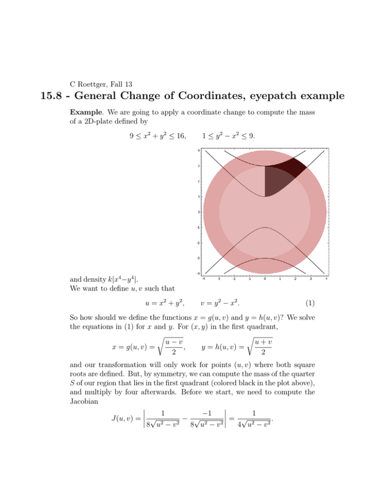
C Roettger, Fall 13
15.8 - General Change of Coordinates, eyepatch example
Example. We are going to apply a coordinate change to compute the mass
of a 2D-plate defined by
9 ≤ x2 + y 2 ≤ 16,
1 ≤ y 2 − x2 ≤ 9.
and density k|x4 −y 4 |.
We want to define u, v such that
u = x2 + y 2 ,
v = y 2 − x2 .
(1)
So how should we define the functions x = g(u, v) and y = h(u, v)? We solve
the equations in (1) for x and y. For (x, y) in the first quadrant,
r
r
u−v
u+v
x = g(u, v) =
,
y = h(u, v) =
2
2
and our transformation will only work for points (u, v) where both square
roots are defined. But, by symmetry, we can compute the mass of the quarter
S of our region that lies in the first quadrant (colored black in the plot above),
and multiply by four afterwards. Before we start, we need to compute the
Jacobian
1
−1
= √ 1
J(u, v) = √
− √
.
8 u2 − v 2 8 u2 − v 2 4 u2 − v 2
We also need to compute our limits for u, v. They are easy! 9 ≤ u ≤ 16 and
1 ≤ v ≤ 9, and R is a rectangle. This already ensures u ≥ v, so g(u, v) is
defined on R. The mass of the lamina is then
ZZ
ZZ
uv
4
4
√
dv du
m = 4k
|x − y | dx dy = 4k
2
2
R 4 u −v
S
Z 9
16
v (u2 − v 2 )1/2 9 dv
= k
Z1 9
v((162 − v 2 )1/2 − (92 − v 2 )1/2 ) dv
= k
1
9
k
= − (256 − v 2 )3/2 − (81 − v 2 )3/2 1
3
k
=
(2553/2 − 803/2 − 1753/2 ).
3
Now that you have made it through this long computation, you should look
again at the picture: