STATISTICS 402B Spring 2016 Homework Set#2 Solution 1.
advertisement
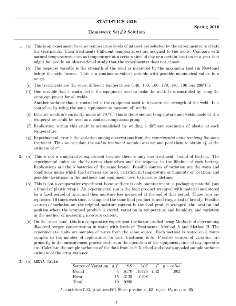
STATISTICS 402B Spring 2016 Homework Set#2 Solution 1. (a) This is an experiment because temperature levels of interest are selected by the experimenter to create the treatments. Then treatments (different temperatures) are assigned to the welds. Compare with natural temperatures such as temperature at a certain time of day or a certain location or a year that might be used in an observational study that the experimenter does not choose. (b) The response variable is the strength of the weld as measured by the maximum load (in Newtons) before the weld breaks. This is a continuous-valued variable with possible nummerical values in a range. (c) The treatments are the seven different temperatures (140, 150, 160, 170, 180, 190 and 200◦ C). (d) One variable that is controlled is the equipment used to make the weld. It is controlled by using the same equipment for all welds. Another variable that is controlled is the equipment used to measure the strength of the weld. It is controlled by using the same equipment to measure all welds. (e) Because welds are currently made at 170◦ C, this is the standard temperature and welds made at this temperature could be used as a control/comparison group. (f) Replication within this study is accomplished by welding 5 different specimens of plastic at each temperature. (g) Experimental error is the variation among observations from the experimental units receiving the same treatment. Thus we calculate the within treatment sample variance and pool them to obtain s2E as the estimate of σ 2 . 2. (a) This is not a comparative experiment because there is only one treatment: brand of battery. The experimental units are the batteries themselves and the response in the lifetime of each battery. Replications are the 5 batteries of the same brand. Possible sources of variation are the ways and conditions under which the batteries are used, variation in temperature or humidity or location, and possible deviations in the methods and equipment used to measure lifetime. (b) This is not a comparative experiment because there is only one treatment: a packaging material (say a brand of plastic wrap). An experimental run is the food product wrapped with material and stored for a fixed period of time, and then moisture loss measured at the end of that period. These runs are replicated 10 times each time, a sample of the same food product is used (say, a loaf of bread). Possible sources of variation are the original moisture content in the food product wrapped, the location and position where the wrapped product is stored, variation in temperature and humidity, and variation in the method of measuring moisture content. (c) On the other hand, this is a comparative experiment the factor studied being Methods of determining dissolved oxygen concentration in water with levels or Treatments: Method A and Method B. The experimenatal units are samples of water from the same source. Each method is tested on 6 water samples so the number of replications for each treatment is 6. Possible sources of variation are primarily in the measurement process such as in the operation of the equipment, time of day, operator etc. Calculate the sample variances of the data from each Method and obtain apooled sample variance estimate of the error variance. 3. (a) ANOVA Table Source of Variation d.f. SS MS F p − value Brand 4 .6170 .15425 7.42 .002 Error 15 .3125 .0208 Total 19 .9295 F -statistic=7.42, p-value=.002 Since p-value < .05, reject H0 at α = .05 1 Best estimates: µ̂1 = ȳ1. = 2.325, µ̂2 = ȳ2. = 2.375, µ̂3 = ȳ3. = 2.05, µ̂4 = ȳ4. = 2.60, µ̂5 = ȳ5. = 2.375 σ̂ 2 = s2E = .0208 (b) Residuals: Brand Acme Champ Ajax Tuffy Xtra −0.025 −0.175 0.15 −0.2 −0.075 0.075 −0.075 −0.05 0.1 0.125 −0.225 0.025 −0.15 0.0 −0.075 0.175 0.225 0.05 0.1 0.025 (c) 95% Confidence Intervals from JMP µ1 − µ2 : (−.2675, .1675) µ1 − µ3 : (.0575, .4925)∗ µ1 − µ4 : (−.4925, −.0575)∗ µ1 − µ5 : (−.2675, .1675) µ2 − µ3 : (.1075, .5425)∗ µ2 − µ4 : (−.4425, −.0075)∗ µ2 − µ5 : (−.2175, .2175) µ3 − µ4 : (−.7675, −.3325)∗ µ3 − µ5 : (−.5425, −.1075)∗ µ4 − µ5 : (.0075, .4425)∗ The CI’s marked with and asterisk do not contain zero; so those pairs of means are significantly different at α = .05 (d) Compute LSD at α = .05: r LSD.05 = t.025,15 sE 2 = t.025,15 n s s 2s2E = 2.131 n 2(.0208) = .2173 4 Arrange the sample means in increasing order of magnitude. The underscoring procedure gives: Brand Ajax Acme Xtra Champ Tuffy Means 2.05 2.325 2.375 2.375 2.6 ——————————– Conclusions: • The data show that Ajax is the brand with the lowest mean wear as measured by weightloss, with significantly lower wear than any other brand. • Acme, Xtra, and Champ have similar wear but significantly larger than Ajax. • Tuffy is found to have largest wear rate significantly larger than all other brands. (e) Compute Tukey’s HSD at α = .05: r T ukey.05 = Q · sE s 2 =Q n 2s2E = 3.08792 n s 2(.0208) = .315 4 Arrange the sample means in increasing order of magnitude: The underscoring procedure gives: Brand Ajax Acme Xtra Champ Tuffy Means 2.05 2.325 2.375 2.375 2.6 —————– ——————————————Conclusions: • Much smaller number of wear means were found to be different. Ajax and Acme were found to have similar wear but significantly smaller weight loss than other three brands. 2 • However, Acme, Xtra, Champ, and Tuffy were also have similar wear but significantly larger weight loss than Ajax. • This is a conflicting result. Thus the only feasible conclusion to be drawn is that Ajax has the smallest wear rate; Xtra, Champ, and Tuffy has significantly larger wear rate, with Acmw in the middle. 4. (a) ANOVA Table Source of Variation d.f. SS MS F p − value Electrolyte 3 550.95 183.65 87.45 < .0001 Error 16 33.60 2.10 Total 19 584.55 Best estimates: µ̂1 = ȳ1. = 33.8, µ̂2 = ȳ2. = 34.4, µ̂3 = ȳ3. = 46.2, µ̂4 = ȳ4. = 42.2 σ̂ 2 = s2E = 2.1 with 16 d.f. (b) Contrast Coefficients: Contrast Label C1 : C2 : C3 : 1 0 .5 Coefficients -1 0 0 1 .5 -.5 0 -1 -.5 (c) It is easy to check that for c1 , . . . , c4 and d1 , . . . , d4 that. 4i=1 ci = 0, 4i=1 di = 0, and holds. Thus C1 , C2 , C3 are contrasts that are also orthogonal to each other. Estimates and Standard errors (from JMP): P (d) Contrast Label C1 : C2 : C3 : 1 0 .5 i. H0 : µ1 = µ2 vs. Coefficients -1 0 0 1 .5 -.5 0 -1 -.5 Estimate -0.6 4.0 -10.1 P P4 i=1 ci di =0 Std. Err. 0.9165 0.9165 0.6481 Ha : µ1 6= µ2 . t-statistic= -0.655 p-value=.522 Fail to Rej. H0 at α = .05 ii. H0 : µ3 = µ4 vs. Ha : µ3 6= µ4 . t-statistic= 4.3644 p-value=0.0005 Rej. H0 at α = .05 iii. H0 : (µ1 + µ2 )/2 = (µ3 + µ4 )/2 vs. Ha : (µ1 + µ2 )/2 6= (µ3 + µ4 )/2. t-statistic= -15.58 p-value=0.0000 Rej. H0 at α = .05 There is no significant difference in mean lifetime between Electrolytes 1 and 2; there is is a significant difference in mean lifetimes between Electrolytes 3 and 4; there is a significant difference in between average of mean lifetimes of Electrolytes 1 and 2 and average of mean lifetimes Electrolytes 3 and 4. Thus the chemical used in Electrolytes 3 and 4 appear to result significantly longer life in automobile batteries. (e) Expanded ANOVA Table incorporating contrasts: Source of Variation d.f. SS MS F p − value Electrolyte 3 550.95 183.65 87.45 < .0001 —– 1 vs. 2 1 0.9 0.9 0.43 0.5 —– 3 vs. 4 1 40.0 40.0 19.0 .0005 —– 1+2 vs. 3+4 1 510.05 510.05 242.88 0.0000 Error 16 33.60 2.10 Total 19 584.55 hline Contrast sums of squares completely partition the treatment sum of squares because three contrast are orthogonal and we have equal sample sizes. We see that SST rt = 550.95 = 0.9 + 40.0 + 510.05 3

