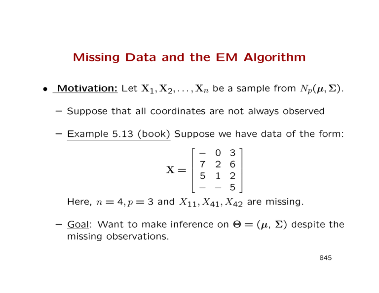
Missing Data and the EM Algorithm
• Motivation: Let X1, X2, . . . , Xn be a sample from Np(µ, Σ).
– Suppose that all coordinates are not always observed
– Example 5.13 (book) Suppose we have data of the form:

X


=

−
7
5
−
0
2
1
−
3
6
2
5





Here, n = 4, p = 3 and X11, X41, X42 are missing.
– Goal: Want to make inference on Θ = (µ, Σ) despite the
missing observations.
845
The “What if” Approach
• Suppose that the observations were actually not missing.
Pn
n
1
Then `(Θ) = − 2 log Σ − 2 i=1(Xi − µ)0Σ−1(Xi − µ) + c and
Θ is chosen to maximize it. This yields the usual MLEs.
• But we do not have some of these observations!
• Provide an iterative scheme with current values for Θ, replace
the missing values by their conditional expectations given the
observed data and the current guesses for Θ.
• The scheme and its theoretical basis is provided next.
846
The EM Algorithm
• Let Y be the observed data, X be the missing data and
Z = (X, Y) be the complete data. We are able to maximize
the complete loglikelihood `(Θ; X, Y) easily but really want
to maximize the observed loglikelihood `(Θ; Y).
• The EM algorithm consists of two steps:
– The E-step: The Expectation step computes the expectation of the complete loglikelihood given observations Y.
i.e., let Θ(i) be the current guess for Θ. The calculate
Q(Θ, Θ(i)) =
Z
`(Θ; X, Y)f (X | Y; Θ(i))dX.
– The M-step: The Maximization step maximizes Q(Θ, Θ(i))
as a function of Θ to get Θ(i+1).
• Iterate till convergence to get MLE Θ̂.
847
Proof of the EM Algorithm - I
• Note that: `(Θ; X, Y) = `(Θ; X | Y) + `(Θ; Y)
• The E-step integrates out the missing parts of the data:
Z
`(Θ; X, Y)dF (X | Y; Θ∗) =
Z
`(Θ; X | Y)dF (X | Y; Θ∗)+`(Θ; Y)
• Thus, we get
`(Θ; Y) = Q(Θ; Θ∗) − H(Θ; Θ∗)
where Q(Θ; Θ∗) is
as before (the calculation in the E-step)
R
and H(Θ; Θ∗) = `(Θ; X, Y)dF (X | Y; Θ∗).
• We show that `(Θ; Y) does not decrease at any iteration.
848
Proof of the EM Algorithm - II
We have `(Θ(i+1); Y) − `(Θ(i); Y) = Q(Θ(i+1); Θ(i)) − Q(Θ(i); Θ(i))
− [H(Θ(i+1); Θ(i)) − H(Θ(i); Θ(i))]
• Note that Q(Θ(i+1); Θ(i)) − Q(Θ(i); Θ(i)) ≥ 0 is true by the
M-step.
• H(Θ(i+1); Θ(i)) − H(Θ(i); Θ(i)) ≤ 0 by Jensen’s inequality.
• This provides a formal proof of the EM algorithm.
849
Initialization and Variance Estimation
• Note that the EM can be very sensitive to initialization.
Pn
(i+1)
(i)
• Write Q(Θ
; Θ ) = i=1 qi(Θ(i+1); Θ(i))
• Then, the observed information matrix at Θ̂n, I(Θ̂; Y), can
be approximated by the empirical information matrix defined
as (∇q1...∇q2... . . . ...∇qn)(∇q1...∇q2... . . . ...∇qn)0| (K)
(K) , where
Θ =Θ̂n
∇qi is the gradient vector of the expected complete log likelihood at the ith observation qi ≡ qi(Θ(K); Yi)
• This makes variance estimation practical in independent identically distributed models.
850