STAT 511
Spring 2002
Assignment 4
Name ________________
Reading Assignment: Rencher: Read Chapters 11, 4 and 5. Chapter 11 was part of an earlier
reading assignment. It covers the basics on estimable functions and
testable hypotheses. Chapter 4 reviews some properties of the multivariate
normal distribution, and Chapter 5 considers distributions of quadratic
forms and related F and t distributions. The introduction to regression
analysis in Chapters 6 and 7 and the regression diagnostics in Chapter 9
were covered in Stat 500, and we will not repeat the coverage of this
material in Stat 511. You can review as much of this material as you find
useful. Chapter 8 covers tests of hypotheses and confidence intervals for
parameters in regression models. Reading Chapter 8 will help you apply
the general linear model theory we are developing in Stat 511 to the
analysis of multiple regression models.
Written Assignment: On-campus students: Due Friday, February 15, in class.
Distance students: Put it in the mail or e-mail or FAX by February 22.
1.
A food scientist performed the following experiment to study the effects of combining
three different fats and three different surfactants on the specific volume of bread loaves.
Four batches of dough were made for each of the six combinations of fat and surfactant.
Ten loaves of bread were made from each batch of dough and the average volume of the
ten loaves was recorded for each batch. Unfortunately, some of the yeast used to make
some batches of dough was ineffective and data from the loaves made from those batches
had to be removed from the analysis. Fortunately, all six combinations of the levels of fat
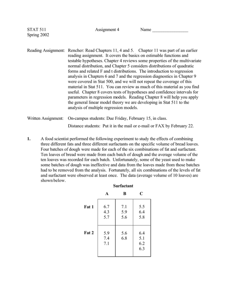
and surfactant were observed at least once. The data (average volume of 10 loaves) are
shown below.
Surfactant
A
B
C
Fat 1
6.7
4.3
5.7
7.1
5.9
5.6
5.5
6.4
5.8
Fat 2
5.9
7.4
7.1
5.6
6.8
6.4
5.1
6.2
6.3
2
Consider the model Yijk = µ + αi + βj + γij + εijk where εijk ~ NID(0, σ 2) and Yijk
denotes the average of the volumes of ten loaves of bread made from the k-th batch of
dough using the i-th fat and the j-th surfactant. For each of the following linear
functions of the parameters, determine if it is estimable. If it is estimable, give a vector
a such that E (a T Y) is equal to that linear combination of parameters. If it is estimable,
describe what that linear combination of parameters represents with respect to the effects
of the fats and surfactants on mean bread volume.
(a) µ
(b) α 2
(c) β 2 − β 3
(d) γ 23
(e) µ + α2 + β 3 + γ 23
(f) γ 11 − γ12
(g) γ 11 − γ 13 − γ 21 + γ 23
(h) (β 2 − β3 ) +
1
( γ12 + γ 22 − γ 13 − γ 23 )
2
(i) γ 12 + γ 22 − γ 13 − γ 23
2. Data were collected to study the effect of temperature on the yield of a chemical process.
Two different catalysts A and B, were used in the study. Yields were measured under 5
different temperatures for each catalyst. The data are as follows:
Run
3
10
4
8
5
9
2
6
1
7
Yield (grams)
Y
20
24
27
33
38
25
29
32
37
41
Temperature (°° C)
T
90
95
100
105
110
90
95
100
105
110
Catalyst
A
A
A
A
A
B
B
B
B
B
3
Each run can be considered as an independent observation. The order in which the runs were
made was randomized.
Consider the linear model
Yij = µ + αi + β(Tij − 100) + ε ij ,
for i = 1, 2 and j = 1, 2, ..., 5
where
Yij = the observed yield for the run using the i-th catalyst and the j-th
temperature level.
αi
correspond s to the i − th catalyst
Tij = the temperature under which the process was run.
(a) For this linear model the vector of mean responses can be written as E(Y ) = X β . Write
out the model matrix X corresponding to the parameter vector â = (µ α1 α 2 β) T .
(b) Determine which, if any, of the following quantities are estimable. For each estimable
quantity, report the value of a vector a such that aTY satisfies the definition of an
estimable function of β .
(i)
µ
(ii)
µ +α2
(iii)
β
(iv)
α1 - α2
(v)
µ+ βT
where T is any specified temperature
(vi)
µ + α1 + β (T-100)
where T is any specified temperature
(c) The data are posted in the file hw402p2.txt on the course web page. This file has five
columns. The first two columns match the first two columns in the table shown above.
The third and fourth column use dummy variables to indicate which catalyst was used.
The third column is coded “1” when catalyst A was used and coded “0” when the other
catalyst was used. The fourth column is coded “1” when catalyst B was used and coded
“0” when the other catalyst is used. The fifth column contains the temperature values
minus 100. Use the command
4
W <-
read.table("c:/stat511/hw402p2.txt",header= T)
to enter these data into a data frame in S-PLUS. Of course, you should replace
"c:/stat511/hw402p2.txt" with the name of the file in which you stored these data.
Use the command
Y <- as.matrix(W[ ,2 ])
to create a vector of observed responses. Use the command
X <- as.matrix(cbind(rep(1,length(Y)),W[ ,3:5]))
to construct the model matrix for the model in part (a).
If you are using S-PLUS version 6 for Windows or the UNIX version 5.1 of S-PLUS
(available on the system of VINCENT workstations at ISU), use the ginverse( ) function
to compute a generalized inverse of XTX and report the result. If you are using an older
version of S-PLUS for windows, the ginverse( ) function will not be available. Those
users can use the ginv( ) function in the MASS library of functions. The MASS library
comes with any Windows version of S-PLUS and you downloaded it onto you computer
when you installed S-PLUS. To use a function in the MASS library, you must first
establish a path to the library by issuing the command
library(MASS)
from the command window. Then when you issue the command
M <- ginv(t(X)%*%X)
S-PLUS will looking the MASS library for the ginv( ) function. If you fail to issue the
library(MASS) command, S-PLUS will only look for the ginv( ) in the default library of
functions.
(d) Use S-PLUS to check if the generalized inverse computed in part (c) satisfies the four
properties of the Moore-Penrose inverse. State your conclusion.
(e) Use the generalized inverse from part (c) to compute a solution to the normal equations
X T Xb = X T Y . Report your value of b .
(f) To visually check if the proposed model is reasonable for these data and to practice
5
using S-PLUS to make plots, create a scatter plot of yield (Y) versus temperature (T).
Use an open circle for the 5 observations with catalyst A and a filled circle for the five
observations with catalyst B. Also include two parallel lines on the plot corresponding to
the least squares estimates of the models for catalysts A and B. This can be done with the
following code.
#
#
Splus code for problem 2 on hw4, 2002
Enter the data into a data frame
W <- read.table("c:/stat511/hw402p2.txt",header=T)
# Create the response vector
Y <- as.matrix(W[,2])
#
Construct a vector of temperatures
temp <- X[ ,4]
# Construct a factor to represent the groups
groups <- as.factor(W[ ,3]+2*W[ ,4])
#
Use the lm( ) function to fit the model
lm.out <- lm(Y~groups+temp)
#
#
#
#
Plot the observations on the same plot
with the estimated lines.
First construct the axes for the plot
and print titles and labels.
par(fin=c(7,7),mar=c(5,5,4,2),cex=1.5,mkh=1.3)
plot(c(min(temp),max(temp)), c(min(Y),max(Y)),
xlab='Temperature-100',ylab='Yield',
type="n", main="Problem 2 on Assignment 4 ")
#
Now insert the observations and fitted lines
pc <- c(1,16)
lt <- c(1,7)
N <- seq(1,length(groups))
for(i in sort(unique(groups))) {
j <- N[groups == i]
points(temp[j], Y[j], pch = pc[i])
lines(temp[j],lm.out$fitted[j],lty=lt[i])
}
Submit your plot and comment on the results.
6
(g) Using your solution b = (µˆ αˆ 1 αˆ 2 βˆ )T to the normal equations from part (c), estimates
of the lines that describe how the mean yield changes with changes in temperature are
Ŷ1 j = µˆ + αˆ 1 + βˆ T1 j
when catalyst A is used
and
Ŷ2 j = µˆ + αˆ 2 + βˆ T2 j when catalyst B is used
Would these estimates change if you used a different solution to the normal equations?
Explain.
3. Consider the “common mean” model Yij = µ + εij , i = 1, 2 and j = 1, 2, ..., 5, for the data
in problem 2. This model can be expressed as Y = 1 µ + ε , where
Y = ( Y11 Y12 Y13 Y14 Y15 Y21 Y22 Y23 Y24 Y25 ) T is vector of observed yields and
1
= (1 1 1 1 1 1 1 1 1 1)T is a model matrix with one column.
(a) Note that µˆ = (1T 1)-1 1T Y is the unique solution to the normal equations for this model.
Show that µˆ = (1T 1) -1 1T Y = Y•• , the sample mean of the ten observations.
(b) Show that P1 = 1(1T1)-11T satisfies the definition of an idempodent matrix.
ˆ = P1Y , as a function of Y .
(c) Give a formula for the vector of estimated means, Y
••
(d) Show that the uncorrected total sum of squares can be partitioned as
SS total, uncorrected = Y T Y = Y T P1Y + YT (I − P1 )Y = SS mod el , uncorrected + SS residuals .
7
2 5
(e) For the “common mean” model, SS residuals = YT (I − P1 )Y = ∑ ∑ (Yij − Y• • )2 , is the
i =1 j=1
quantity that one generally calls the corrected total sum of squares. Obtain a formula for
SS mod el, uncorrected = Y T P1Y as a function of Y•• .
(f) Show that the uncorrected total sum of squares can also be partitioned as
SS total, uncorrected = Y T Y = Y T P1Y + YT (PX − P1 )Y + Y T ( I − PX )Y , where PX is the
projection matrix for the model in problem 2.
(g) Show that the corrected model sum of squares for the model in problem 2 is
SS mod el , problem 2 = YT (PX − P1 )Y = SS residuals, common means model - SSresiduals, problem 2
the difference between the residual sum of squares for the “common means” model and
the model in problem 2. The degrees of freedom for this sum of squares is the difference
in the dimensions of the residual spaces for the two models, i.e., (10-1)-(10-3)=2 d.f..