Inference in Linear Regression
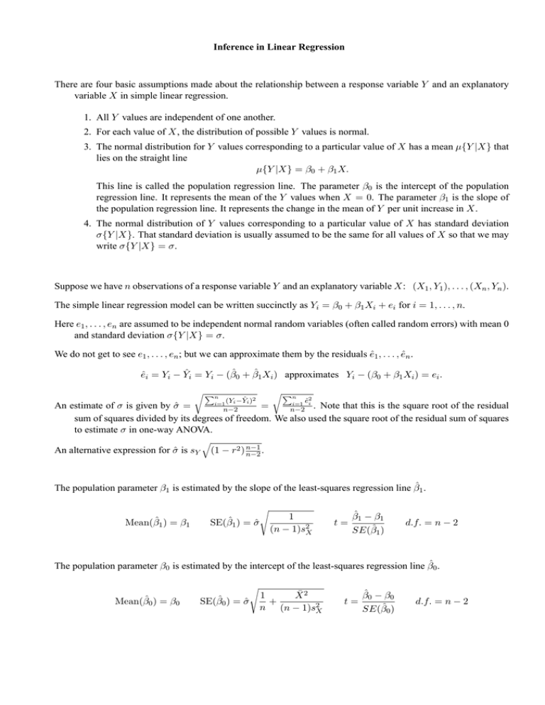
There are four basic assumptions made about the relationship between a response variable Y and an explanatory
variable X in simple linear regression.
1. All Y values are independent of one another.
2. For each value of X, the distribution of possible Y values is normal.
3. The normal distribution for Y values corresponding to a particular value of X has a mean µ{Y |X} that
lies on the straight line
µ{Y |X} = β0 + β1 X.
This line is called the population regression line. The parameter β0 is the intercept of the population
regression line. It represents the mean of the Y values when X = 0. The parameter β1 is the slope of
the population regression line. It represents the change in the mean of Y per unit increase in X.
4. The normal distribution of Y values corresponding to a particular value of X has standard deviation
σ{Y |X}. That standard deviation is usually assumed to be the same for all values of X so that we may
write σ{Y |X} = σ.
Suppose we have n observations of a response variable Y and an explanatory variable X: (X1 , Y1 ), . . . , (Xn , Yn ).
The simple linear regression model can be written succinctly as Yi = β0 + β1 Xi + ei for i = 1, . . . , n.
Here e1 , . . . , en are assumed to be independent normal random variables (often called random errors) with mean 0
and standard deviation σ{Y |X} = σ.
We do not get to see e1 , . . . , en ; but we can approximate them by the residuals ê1 , . . . , ên .
êi = Yi − Ŷi = Yi − (β̂0 + β̂1 Xi ) approximates Yi − (β0 + β1 Xi ) = ei .
rP
rP
n
(Y −Ŷi )2
i=1 i
n
ê2
i=1 i
An estimate of σ is given by σ̂ =
=
n−2
n−2 . Note that this is the square root of the residual
sum of squares divided by its degrees of freedom. We also used the square root of the residual sum of squares
to estimate σ in one-way ANOVA.
An alternative expression for σ̂ is sY
q
(1 − r2 ) n−1
n−2 .
The population parameter β1 is estimated by the slope of the least-squares regression line β̂1 .
Mean(β̂1 ) = β1
SE(β̂1 ) = σ̂
s
1
(n − 1)s2X
t=
β̂1 − β1
SE(β̂1 )
d.f. = n − 2
The population parameter β0 is estimated by the intercept of the least-squares regression line β̂0 .
Mean(β̂0 ) = β0
SE(β̂0 ) = σ̂
s
1
X̄ 2
+
n (n − 1)s2X
t=
β̂0 − β0
SE(β̂0 )
d.f. = n − 2
Using data from 56 U.S. cities collected from 1931 to 1960, we computed the equation of the least-squares regression line relating average minimum January temperature (Y ) to latitude in degrees north of the equator (X) as
Ŷ = 108.56 − 2.104X. To determine the equation of the least-squares regression line we used the following
summary statistics:
X̄ = 39.0
Ȳ = 26.5
SX = 5.4
SY = 13.4
r = −0.848.
Use this information to help you complete the following problems.
1. Estimate β0 .
2. Estimate β1 .
3. Compute a 95% confidence interval for β1 .
4. Is there a significant linear relationship between average minimum January temperature and latitude? Test
H0 : β1 = 0 against HA : β1 6= 0.
5. Which of the four assumptions of simple linear regression can you check by examining a scatter plot of Y vs.
X? Do any of the assumptions that you can check appear to be violated?