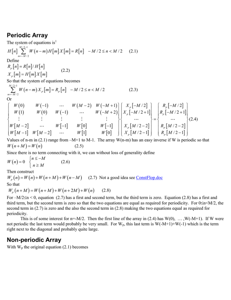
Periodic Array
The system of equations is1
H  n
M / 2 1

m  M / 2
W  n  m  H  m X  m  R  n  M / 2  n  M / 2
(2.1)
Define
Rp  n  R  n / H  n
(2.2)
X p  m  H  m X  m
So that the system of equations becomes
M / 2 1

m  M / 2
W  n  m  X p  m  Rp  n  M / 2  n  M / 2
(2.3)
Or
W  1
W  M  2  W   M  1   X p   M / 2   R p   M / 2 
 W  0
 



W  0
W  1
W   M  2    X p   M / 2  1  R p   M / 2  1
 W 1


 




 (2.4)
W  M  2




X  M / 2  2
R  M / 2  2 
W  1
W  0
W  1

 p
  p

W 1
W  0   X p  M / 2  1   R p  M / 2  1 
W  M  1 W  M  2
Values of n-m in (2.1) range from –M+1 to M-1. The array W(n-m) has an easy inverse if W is periodic so that
(2.5)
W  n  M   W  n
Since there is no term connecting with it, we can without loss of generality define
n   M
W  n  0 
(2.6)
nM
Then construct
Wp  n   W  n   W  n  M   W  n  M  (2.7) Not a good idea see ConstFlop.doc
So that
(2.8)
Wp  n  M   W  n  M   W  n  2M   W  n 
For –M/2n < 0, equation (2.7) has a first and second term, but the third term is zero. Equation (2.8) has a first and
third term, but the second term is zero so that the two equations are equal as required for periodicity. For 0n<M/2, the
second term in (2.7) is zero and the also the second term in (2.8) making the two equations equal as required for
periodicity.
This is of some interest for n=-M/2. Then the first line of the array in (2.4) has W(0), … ,W(-M+1). If W were
not periodic the last term would probably be very small. For Wp, this last term is W(-M+1)+W(-1) which is the term
right next to the diagonal and probably quite large.
Non-periodic Array
With Wp the original equation (2.1) becomes
H  n
M / 2 1

m  M / 2
 H  n
Wp  n  m  H  m X  m 
M / 2 1

m  M / 2
W  n  M  m  H  m X m  H n 
M / 2 1

m  M / 2
(3.1)
W  n  M  m  H m  X m   R n 
Divide by H[n]
M / 2 1

m  M / 2

Wp  n  m  H  m X  m 
M / 2 1

m  M / 2
W  n  M  m  H  m X  m 
M / 2 1

m  M / 2
W  n  M  m  H  m  X  m   R  n  / H [n ]
Multiply by the inverse of Wp(k-n) and sum over n
M / 2 1

m  M / 2
H  m X  m
M / 2 1

n  M / 2
W p1  k  n W p  n  m  
M / 2 1


m  M / 2
So that defining
X p k  
M / 2 1

n  M / 2
Wp1  k  n 
R  n
M / 2 1

m  M / 2
H  m X  m
H m X m
M / 2 1

W
n  M / 2
1
p
M / 2 1

n  M / 2
W p1  k  n W  n  m  M 
M / 2 1
 k  n W  n  m  M   
n  M / 2
W
1
p
k  n
R  n
(3.2)
H  n
(3.3)
H  n
Equation (3.2) becomes
H k  X k   H k  X p k  
M / 2 1

m  M / 2
H m X m
M / 2 1

n  M / 2
W p1  k  n  W  n  m  M   W  n  m  M  
(3.4)
This is true for any X[m]. In fact given any X[m] it generates a new approximation to X[m] so that one could iterate as
H  k  X it  k   H  k  X p  k  
M / 2 1

m  M / 2
H  m  X it 1  m 
M / 2 1

n  M / 2
W p1  k  n  W  n  m  M   W  n  m  M  
(3.5)
The sums are convolutions with
ws  ti  
M / 2 1
 W  m  M   W  m  M   exp   j 2 f t 
m i
m  M / 2
ti 
Ti
m
; fm 
(3.6)
M
T
And
hxit 1  ti  
M / 2 1

m  M / 2
H  m  X it 1  m  exp   j 2 f m ti 
ti 
Ti
m
; fm 
M
T
(3.7)
Note that time is defined in terms of T/M, not T/N.
1 M / 21
T
H  m X it 1  m  W  n  m  M   W  n  m  M   

T m M / 2
M
(3.8)
Then with
wp1  ti  
M / 2 1

m  M / 2
W p1  m  exp   j 2 f m ti 
1 M / 21 1
T
Wp  k  n  HWs X it 1  n  

T n  M / 2
M

i  M / 2
hxit 1  ti  ws  ti  exp  j 2 f m ti   HWs X it 1  f m 
(3.9)
M / 2 1

M / 2 1
i  M / 2
hws xit 1  ti  wp1  ti  exp  j 2 f k ti 
(3.10)
The FFT’s in (3.6) and (3.9) need to be made once for every new choice of M. The FFT’s in (3.7) and (3.10) need to
be made for every iteration. Since this starts from (3.1) which is merely a restating of (2.1), and X[m] can be used as
the first iteration.
Finally
(3.11)
H  k  X it  k   H  k  X p k   HWs X it 1Wp1 k 
Diagonal Array
Define W hat to be all but the diagonal terms of W
W  n  Wd 0  Wˆ  n
With Wd the original equation (2.1) becomes
H  n
M / 2 1

m  M / 2
Wd  0  m,n H  m  X  m   H  n 
M / 2 1

m  M / 2
W  n  m  H m  X m   R n 
(4.1)
Multiply by the inverse of Wd(k-n) and sum over n
M / 2 1

n  M / 2
H  n Wd1 k ,n
M / 2 1

m  M / 2
Wd  0 m,n H  m  X  m  
M / 2 1

n  M / 2
H  n Wd1 k ,n
M / 2 1

m  M / 2
W  n  m  H m  X m  
M / 2 1

n  M / 2
Wd1 k ,n R n 
(4.2)
So that
H  k  H  k  X  k   H  k Wd1
M / 2 1

m  M / 2
W  k  m  H  m  X  m   Wd1 R  k 
(4.3)
So that as an iterative method
H  k  X it  k   Wd1 R  k  / H  k   Wd1
M / 2 1

m  M / 2
W  k  m  H  m  X it 1  m 
(4.4)
This is true for any X[m]. In fact given any X[m] it generates a new approximation to X[m] so that one could iterate as
The sums are convolutions with
M / 2 1
Ti
m
wˆ  ti    Wˆ  m  exp   j 2 f m ti 
ti 
; fm 
(4.5)
M
T
m  M / 2
And
M / 2 1
Ti
m
hxit 1  ti    H  m  X it 1  m  exp   j 2 f m ti 
ti 
; fm 
(4.6)
M
T
m  M / 2
Note that ti is defined in terms of T/M, not T/N.
ˆ
H  k  X it  k   Wd1 R  k  / H  k   Wd1  WHX
it 1  k  (4.7)
Error in the solution
The set of equations (2.1) arises from minimizing 2. The R[n] is the derivatives of 2 with respect to the n’th
coefficient. In a first order expansion
 2   02 
M / 2 1
 D
n  M / 2
n
 Dn ,0  R  n 
(5.1)
Assume that the error in the final steps is dominated by the error in solving for Dn-Dn.0 rather than from truncation of
the expansion in (5.1).
After solving for X n = Dn-Dn,o
H  n
M / 2 1

m  M / 2
W  n  m  H  m X  m  R  n   n
(5.2)
So that after the final step
 2   02 
M /2

n  M / 2
 m  n
Mixing
Equations (3.11) and (4.7) generate new solutions from old. In addition there are tridiagonal and band methods
for truncating W to a few bands in (2.4) to generate solutions, but no inverse. It makes sense to combine all of these
with a set of adjustable coefficients to give the best fit. One extra twist, the periodic solutions should be best in the
middle, thus include it with apexp(-(4fm/MT)2) so that it is weighted towards the middle of the integration region.
Find a1 to ak by minimizing

2
err

M / 2 1

n  M / 2
 n  a   n  a 
(6.1)
 K

W
n

m
H
m

     ak X k  m   R n    n  a  (6.2)

m  M / 2
 k 1

Each sum over M is a convolution
1 M / 21
T M / 21
W
n

m
H
m
X
m

   k 
 
 w  ti  hx  ti  exp  j 2 f n ti  (6.3)
T m  M / 2
N i  M / 2
So that
H  n
M / 2 1
K
T H  n   ak W  HX k   n   R  n    n  a 
(6.4)
k 1
Then
2
M / 2 1 
 err
n a
 
 n  a   c.c. (6.5)
ak ' n  M / 2 ak '
And

2
M / 2 1 
 2  err
n  a   n  a 
 
 c.c.
(6.6)
ak ' ak '' n  M / 2 ak '
ak ''
There are K2 terms in (6.6). The equation to solve is
2
2
K
 2  err
 err
a


(6.7)

k
ak
k '1 ak ' ak '
The matrix is symmetric and positive definite so Cholesky matrix inversion is appropriate.
For very large arrays M  103-6, so that K ~ 102 is appropriate.
In practice this allows us to start with Xp, Xtridiagonal, and Xshort band. These are solved using 7 for the best starting array,
which is then used in (3.11) to generate a new X which can be added to the mixture.
1
This system equations usually occurs as part of Newton Raphson iteration. In this case the R is the set of residuals which is constantly getting
smaller. These interact a bit to the approximation of X below causing one set to want a band like solution and the next set to want a periodic
solution. Also since R is in principly going to zero, highly accurate solutions at each step are not needed.