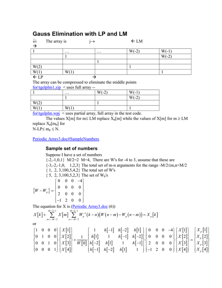
Gauss Elimination with LP and LM
i

1
The array is
 LM
j
…
1
…
W(-2)
W(-1)
W(-2)
1
W(2)
1
W(1)
W(1)
1
 LP

The array can be compressed to eliminate the middle points
for\tgelplm1.zip < uses full array -1
…
W(-2)
W(-1)
1
W(-2)
W(2)
1
W(1)
W(1)
1
for\tgelplm.wpj < uses partial array, full array in the test code.
The values X[m] for m LM replace Xp[m] while the values of X[m] for m  LM
replace Xp[mp] for
N-LP mp  N.
Periodic Array3.doc#SampleNumbers
Sample set of numbers
Suppose I have a set of numbers
{-2,-1,0,1} M/2=2 M=4, There are W's for -4 to 3, assume that these are
{-3,-2,-1,0, 1,2,3} The total set of m-n arguments for the range -M/2m,n<M/2
{ 1, 2, 3,100,5,4,2} The total set of W's
{ 5, 2, 3,100,5,2,3} The set of Wp's
 0 0 0 4 
0 0 0 0
W  Wp    2 0 0 0 


1 2 0 0 
The equation for X is (Periodic Array3.doc (6))
X k  
or
1
0


0
0
M / 2 1

m  M / 2
X  m
M / 2 1

n  M / 2
W p1  k  n  W  n  m   W p  n  m    X p  k 
 1
h  1 h  2 h 1   0
0 0 0   X 1 





1
h  1 h  2  0
1 0 0   X  2 
1  h 1




1
h  1   2
0 1 0   X 3  W  0 h  2 h 1
 h  1 h  2 h 1
1  1
0 0 1   X  4

0 0 4   X 1   X p 1 


 
0 0 0   X  2  X p  2



0 0 0   X 3  X p 3
2 0 0   X  4  X p  4
Multiplying the two 4 x 4 matrices
 1
h  1 h  2 h 1   0


1
h  1 h  2  0
 h 1


1
h  1   2
h  2 h 1
 h  1 h  2 h 1
1  1

0 0 4  2h  2  h  1 2h 1

0 0 0  2h  1  h  2 2h  2 

2h  1
0 0 0   2  h  1
2
2 0 0   2h  1  1


0 4h 1 

0 4h  2 
0 4h  1 
0
4
Adding the diagonal matrix
2h  2  h  1  W  0
  X 1   X p 1 
2h 1
0
4



 
2h  1  h  2
2h  2   W  0 
0
4h 1
1 
  X  2   X p  2




2  h  1
2h  1
W  0
4h  2
W  0 
  X 3   X p 3 

2h  1  1
2
0
4h  1  W  0  X  4  X p  4

Writing out the 4 equations
 2h  2  h  1 
2h 1
4
 1 X 1 
X  2  0 X 3 
X  4  X p 1

W
0
W
0
W
0








 2h  2 
2h  1  h  2
4h 1
X 1  
 1 X  2  0 X 3 
X  4  X p  2
W  0
W  0
 W  0

2  h  1
2h  1
4h  2
X 1

X  2  X 3 
X  4  X p 3
W  0
W  0
W  0
2h  1  1
W  0
 4h  1 
2
X  2  0 X 3  
 1 X  4  X p  4
W  0
 W  0

X 1 
X[3] does not enter into the equations for X[1], X[2], and X[4]. These can be determined
from
2h  2  h  1  W  0
  X 1   X p 1 
2h 1
4
1 


 
2h  1  h  2
2h  2  W  0
4h 1

  X  2   X p  2 
W  0 
2h  1  1
2
4h  1  W 0  X  4   X p  4 

Then the equation for X[3] is
X 3 
X p 3 
M / 2 1

n  M / 2, n 3
X  n Wp1 W  Wp 
n ,3
Wp1 W  Wp 

 3,3
The large diagonal element is left out of the numerator and dominates the denominator.
There is, however, some change to all elements of X.