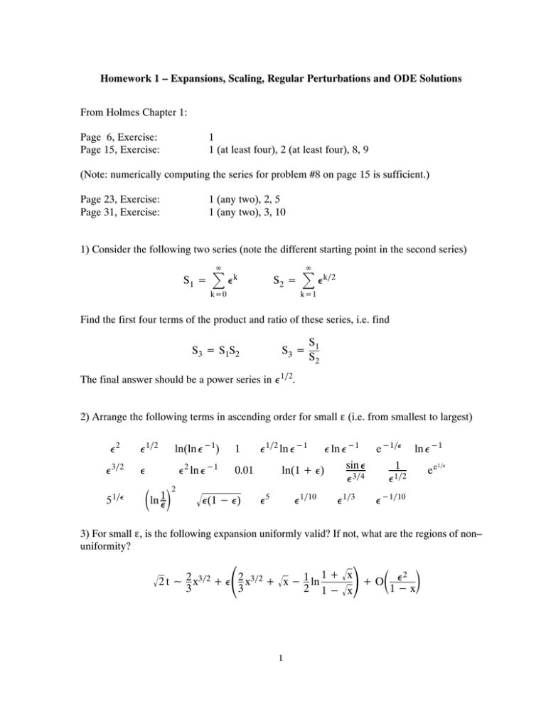
Homework 1 – Expansions, Scaling, Regular Perturbations and ODE Solutions
From Holmes Chapter 1:
Page 6, Exercise:
Page 15, Exercise:
1
1 (at least four), 2 (at least four), 8, 9
(Note: numerically computing the series for problem #8 on page 15 is sufficient.)
Page 23, Exercise:
Page 31, Exercise:
1 (any two), 2, 5
1 (any two), 3, 10
1) Consider the following two series (note the different starting point in the second series)
S1 +
R
ȍ
k
S2 +
k+0
R
ȍ kń2
k+1
Find the first four terms of the product and ratio of these series, i.e. find
S 3 + S 1S 2
S3 +
S1
S2
The final answer should be a power series in 1ń2.
2) Arrange the following terms in ascending order for small (i.e. from smallest to largest)
2
3ń2
5 1ń
1ń2
ln(ln *1)
2 ln *1
ǒln 1Ǔ
2
1
1ń2 ln *1
0.01
Ǹ(1 * )
ln(1 ) )
5
1ń10
ln *1
sin 3ń4
1ń3
e *1ń
ln *1
1
ee
1ń2
1ń
*1ń10
3) For small is the following expansion uniformly valid? If not, what are the regions of non–
uniformity?
ǒ
Ǔ
ǒ
Ǔ
Ǹ
Ǹ2 t X 2 x 3ń2 ) 2 x 3ń2 ) Ǹx * 1 ln 1 ) x ) O 2
3
3
2 1 * Ǹx
1*x
1
4) What values of n give the following results for small :
n Ơ ln n X O(ln )
n ơ ln 5) Consider the following differential equation
dy
)y+0
dt
y(0) + 1
a) Solve this equation exactly
b) Write a Crank–Nicholson algorithm to solve the problem
c) Write a Runge–Kutta algorithm to solve the problem
d) Compare your computed solutions with the exact solution
Hint: Be sure to grid refine each of the computed solutions. Grid refinement is required to determine the grid spacing needed for an accurate solution, and will also help to catch coding errors.
Note: These codes should be saved and used later to assess the qualitative behavior of problems,
prior to doing a perturbation methods solution.
6) Consider the following differential equation
dy
) y2 + 0
dt
y(0) + 1
a) Solve this equation exactly
b) Write a Crank–Nicholson algorithm to solve the problem
c) Write a Runge–Kutta algorithm to solve the problem
d) Compare your computed solutions with the exact solution
Hint: Just use the algorithms developed for problem #5. The Runge–Kutta algorithm requires
minor changes. The Crank–Nicholson algorithm requires a Newton linearization and an extra
iteration loop.
2
7) Many of the initial value problems you will solve involve second order equations. Consider
the projectile problem given in the book:
d 2y
1
+*
2
dt 2
(1 ) y)
y(0) + 0
y Ȁ(0) + 1
a) Write a Crank–Nicholson algorithm to solve the problem
b) Write a Runge–Kutta algorithm to solve the problem
c) Solve the problem using the perturbation method given in the book
d) Compare your computed solutions with the perturbation solution for different values of Note: Make sure that your computed solutions are grid refined!
Hint: This problem has to be written as two equations in two unknowns. The Runge–Kutta algorithm is a straightforward extension of the single equation algorithm. The Crank–Nicholson
method requires a matrix inversion in addition to the differencing and Newton linearization.
Note that the Newton linearization is more complicated than in the previous problem.
8) Consider the boundary value problem given in the book
y ȀȀ ) 2y Ȁ ) 2y + 0
y(0) + 0
y(1) + 1
a) Find the exact solution of this problem
b) Write a central differenced Thomas algorithm to solve the problem
c) Compare your computed solution with the exact solution
d) Compare the exact and computed solutions with the outer solution given in the book
e) Compare the exact and computed solutions with the inner solution given in the book
Hint: When comparing the computed and exact solutions with the perturbation solution you
should plot the perturbation solution on it’s own scales and then plot the exact and computed
solutions on those scales for different values of Note that for this problem, nothing special
needs to be done for the outer solution. However, the plots of the inner solution require a re–scaling of x in the exact and computed solutions in order to get those solutions onto the inner region
scale. You should: a) examine how the computed and exact solutions approach the perturbation
solution as tends to zero, b) figure out exactly how small must be for the perturbation solution
to be accurate, and c) examine the matching between the inner and outer regions.
3