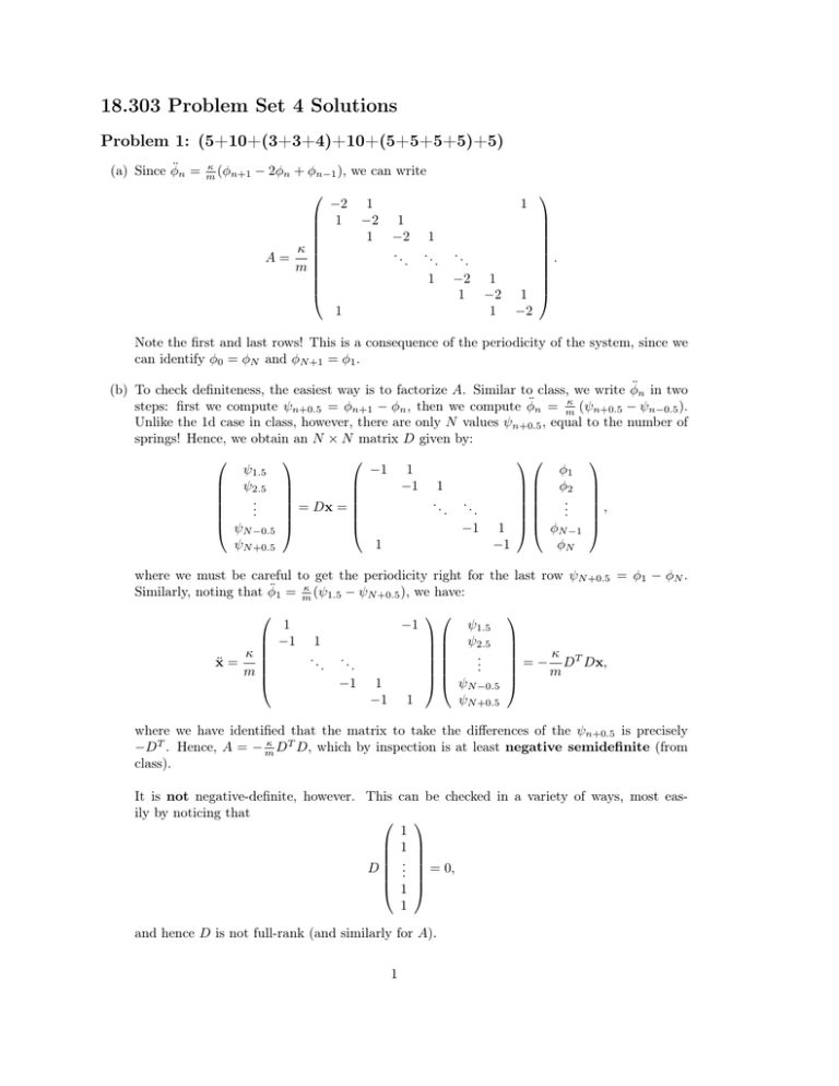
18.303 Problem Set 4 Solutions
Problem 1: (5+10+(3+3+4)+10+(5+5+5+5)+5)
(a) Since φ̈n =
κ
m (φn+1
− 2φn + φn−1 ), we can write

−2
 1


κ 

A=

m



1
1
−2
1
1
1
−2
..
.
1
..
.
1
..
.
−2
1
1
−2
1






.



1 
−2
Note the first and last rows! This is a consequence of the periodicity of the system, since we
can identify φ0 = φN and φN +1 = φ1 .
(b) To check definiteness, the easiest way is to factorize A. Similar to class, we write φ̈n in two
κ
steps: first we compute ψn+0.5 = φn+1 − φn , then we compute φ̈n = m
(ψn+0.5 − ψn−0.5 ).
Unlike the 1d case in class, however, there are only N values ψn+0.5 , equal to the number of
springs! Hence, we obtain an N × N matrix D given by:





ψ1.5
φ1
−1 1
 ψ2.5 
  φ2 

−1 1










..
..
..
..
=
Dx
=



,


.
.
.
.





 ψN −0.5 



φN −1 
−1 1
1
−1
φN
ψN +0.5
where we must be careful to get the periodicity right for the last row ψN +0.5 = φ1 − φN .
κ
Similarly, noting that φ̈1 = m
(ψ1.5 − ψN +0.5 ), we have:

1
 −1
κ 

ẍ =

m

−1
1
..
.
ψ1.5
ψ2.5
..
.





  ψN −0.5
1
ψN +0.5
..
.
−1

1
−1



κ

 = − DT Dx,

m

where we have identified that the matrix to take the differences of the ψn+0.5 is precisely
κ
−DT . Hence, A = − m
DT D, which by inspection is at least negative semidefinite (from
class).
It is not negative-definite, however. This can be checked in a variety of ways, most easily by noticing that


1
 1 




D  ...  = 0,


 1 
1
and hence D is not full-rank (and similarly for A).
1
(c) We defined the rotation operator R by



φ1
φ2
..
.



R

 φN −1
φN

φ2
φ3
..
.



.


 
 
 
=
 
  φN
φ1
(i) By inspection, R is the permutation matrix:

0



R=



1
0
1
..
.



.

1 
0
..
.
0
1
(ii) There are a variety of ways to show this, but the simplest is probably to note that

0
 1


T
R =



1
0
1
..
.
..
.








0
1
0
performs the permutation

φ1
φ2
..
.



R 

 φN −1
φN
T


φN
φ1
..
.
 
 
 
=
 
  φN −2
φN −1




,


which is the rotation in the opposite direction compared to R. Hence, the two operations
cancel one another out and RT R = I.
(iii) Multiplying RA acts R on each of the columns of A, i.e. it permutes each column, giving:

1



κ 

RA =

m


 1
−2
−2
1
1
−2
..
.

1
..
.
1
1
..
.
−2
1
1
−2
1





.

1 

−2 
1
Multiplying AR = (RT AT )T = (RT A)T is equivalent to permuting each row of A by RT
2
(i.e. in the opposite direction), hence

1




κ

RT A =

m


 1
−2
−2
1

1
−2
..
.
1
..
.
..
.
−2
1
1
1
−2
1
1





,

1 

−2 
1
which = RA. Q.E.D.
(d) Consider the vector y = Rx. Using RA = AR, we obtain: Ay = ARx = RAx = λRx =
λy. Therefore, y is an eigenvector of A with eigenvalue λ. But we were told that λ has
multiplicity 1: this means that y must be linearly dependent on x, i.e. y = αx for some
scalar α. Hence y = Rx = αx, and x is an eigenvector of R with eigenvalue α. Q.E.D.
(e) Let Rx = αx.
(i) We need to use the fact that R∗ R = I. Therefore, consider x∗ x = x∗ R∗ Rx = (Rx)∗ (Rx) =
(αx)∗ (αx) = |α|2 x∗ x. Since x∗ x 6= 0 (eigenvectors are nonzero), this means |α|2 = 1,
hence α = eik for some real k.
(ii) We just write out Rx = eik x:

1
x2
..
.



R

 xN −1
xN


x2
x3
..
.
 
 
 
=
 
  xN
1


1
x2
..
.





ik 
=e 



 xN −1
xN







and hence x2 = eik , x3 = eik x2 = e2ik , and so on, or

1
eik
..
.



x=

 ei(N −2)k
ei(N −1)k




,


or more simply:
xn = ei(n−1)k .
(iii) On an eigenvector, RN x = eiN k x = x, and hence eiN k = 1. This means that N k is an
integer multiple of 2π, i.e. N k = 2πm for m = 0, 1, 2, . . ., giving eigenvalues
αm = ei
2πm
N
.
A little more carefully, we notice that αN = α0 , so we have N distinct eigenvalues
m = 0, 1, . . . , N − 1 .
3
(iv) Now that we know the eigenvectors xn , we can plug it back into Ax = λx. Each row of
this equation has the form
κ
(xn+1 − 2xn + xn−1 ) = λxn
m
and plugging in the form of xn = eik(n−1) = eikn e−ik and dividing both sides by xn
gives:
κ
κ ik
e − 2 + eik = λ =
[2 cos(k) − 2] .
m
m
Hence, plugging in the equation for k from above, we have:
λm
2κ
4κ
=
[cos(2πm/N ) − 1] = − sin2
m
m
2πm
N
for m = 0, 1, . . . , N − 1 , where we have used the half-angle identity 1 − cos(k) =
2 sin2 (k/2) to simplify the final expression. Note that the eigenvalues are real and ≤ 0
as expected, with exactly one zero eigenvalue λ0 = 0.
i∆θm(n−1)
(f) The angular difference between each mass is ∆θ = 2π
= eimθ
N , and hence xn = e
where we define the angle θ = (n − 1)∆θ. Hence the eigenfunctions in the continuum limit
are simply
φ(θ) = eimθ
for integers m (or any constant multiple thereof, of course).
Problem 2: (15+10+5+5)
See also the IJulia notebook posted with the solutions.
(a) Setting the slopes to be zero at R1 and R2 simply gives
0
αJm
(kr) + βYm0 (kr) = 0
at the two radii, or E
α
β
= 0 where
E=
0
(kR1 ) Ym0 (kR1 )
Jm
0
Jm (kR2 ) Ym0 (kR2 )
.
Hence, writing fm (k) = det E, we get
0
0
fm (k) = Jm
(kR1 )Ym0 (kR2 ) − Jm
(kR2 )Ym0 (kR1 ) .
Given a k for which fm (k) = 0, then we can solve for the nullspace of E by arbitrarily
choosing
α
a scaling such that α = 1 and solving for β from the first or second rows of E
= 0:
β
β=−
0
Jm
(kR1 )
J 0 (kR2 )
= − m0
.
0
Ym (kR1 )
Ym (kR2 )
(b) The plot is shown in Figure 1. Note that fm (k) for m > 0 has a divergence as k → 0, so we
used the ylim command to rescale the vertical axis (otherwise it would be hard to read the
plot!); see the solution IJulia notebook.
4
f0 (k)
f1 (k)
f2 (k)
0.4
fm (k)
0.2
0.0
0.2
0.4
0
5
10
k
15
20
Figure 1: Plot of fm (k) for m = 0, 1, 2.
(c) We’ll use the Scilab newton function, similar to class, to find the roots, with initial guesses
provided by our plot in Figure 1. We find k1 ≈ 3.196578, k2 ≈ 6.31234951, and k3 ≈
9.4444649. See the solutions notebook.
(d) See the IJulia notebook. Using our k1 and k2 from part (c) and our α and β from part (a),
RR
we find that R12 ru0,1 (r)u0,2 (r)dr ≈ 10−15 , which is zero up to roundoff errors.
5