291205716
1/5
This is a version of MonteCarlo.htm that takes into account
../Tcheby.htm#GaussThebyshevQuadrature – and
../Tcheby.htm#WaitAMinute -- The Fortran code in the links
has not yet been changed. When changed the links will be to
forMod\...
At a glance this says that selecting  in the first
integral rather than the more traditional  changes a
mid-point trapezoidal rule from convergence with 1/N
to Gauss Thebyshev with exponential convergence.
Biased Selection Monte Carlo
The traditional beginning is to consider a 3d integral
over all space
1
1

0
0
0
 f   d rf  r   4  d   d   r 2 f (r )dr
3
  2  1
  2
(1.1)
Change this to
1
1

0
0
0
 f   d rf  r   4  d  d  sin   r 2 f (r )dr
3
  
  2
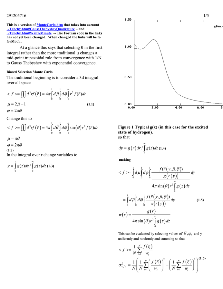
Figure 1 Typical g(x) (in this case for the excited
state of hydrogen).
so that

dy  g  r  dr /  g ( z )dz (1.4)
(1.2)
0
In the integral over r change variables to
r

0
0
y   g ( z )dz /  g ( z )dz (1.3)
making
1
1
1
0
0
0
f (r  y,  ,  )
 f   d   d  
dy
g  r  y 

4 sin   r 2  g  z  dz
1
1
f (r  y,  ,  )
1
  d   d 
0
wr  
0
w  r  y 
0
0
dy
(1.5)
g r 

4 sin   r 2  g  z  dz
0
This can be evaluated by selecting values of  ,  , and y
uniformly and randomly and summing so that
 f 
 2 f 
1
N
N
f  ri 
i 1
wi

11
 
NN

 f  ri    1

 

i 1  wi
 N
N
2
N

i 1
f  ri  

wi 
2




(1.6)
291205716
Note that the 1/r2 in the denominator of w, more than
cancels the typical 1/r in a Coulomb potential. This is
exactly the cancellation that occurs when this potential
is evaluated in spherical coordinates. What has
happened is that the probability of selecting a point
with small r, is much larger when selected uniformly in
spherical coordinates than it is in Cartesian coordinates.
Since g(r) is at our disposal, this can be made as high as
we want in practice.
The detail of actually finding r(y) needs to be
mentioned. To be specific, the values of g are saved and
the straight lines connecting these values become the
actual weight function. This makes w(r) the integral of
forms ai+bir and hence a quadratic in r which requires
solving a quadratic equation for the value of r once y
has been chosen.
2/5
w over the possible ways in which the point could have
been selected. Be very careful, it is rigorous when
done correctly but fraught with possible errors. In this
case the point (x,y,z)i can be chosen either with respect
to R1 with probablility w11 which is given by


w11  g ( r1  R1 ) /  g (  )d  / 4 sin 1  r1  R1
(1.7)
or with respect to R2


w12  g ( r1  R2 ) /  g (  )d  / 4 sin 1  r1  R2
2

2

(1.8)
The average probability is then
 g ( r  R ) / g (  )d  / 4 sin   r  R 2 
1
2
1
1
2

/2
w1  

2 
  g ( r1  R1 ) /  g (  )d  / 4 sin 1  r1  R1 
(1.9)
--The new term in 1 does not really effect the average,
but the vector R1-R2 is a natural choice for its selection.
Note that when the Monte-Carlo picks the same f, but
with different w’s, The average is <1/w> accounting of
course for the relative frequency of selecting the
different (x,y,z)’s. In this case where I definitely did
not wait for an unlikely, small w, event, but noted
analytically that it should be there, the average is of
<w>. Note that when the argument of v(r1-R1) is small
that there is a 1/(r1-R1)2 in the in the denominator of w1
which becomes the numerator of the sum term and
multiplies the singularity to zero and that the same also
happens for r1-R2.
We are not done with w. It is also possible to select
from a random set of points. One estimates the sum as






I
S I  (1/ M ) G (( x, y, z )i ) (1.10)
i 1
Figure 2 normalized integral of g(r)
Graphically the method for going from y to x is shown
above in the plot of w(x) versus x. A y is chosen
randomly between 0 and 1, shown here as being about
.32, and the x corresponding to it is taken as x(y),
shown here as about 1.5.
Of immense practical use
in systems with two singular centers v(r1) and v(r2),
both of which go as 1/r, is the fact that we can average
then a random number, , is chosen. The value (x,y,z)i
for which SI-1 <  < SI has relative probability
g((x,y,z)i)/SM of selection, introducing
wi  G(( x, y, z )i ) / SM .(1.11)
In fact the values in the sum, could themselves have
been chosen with a bias w1i which case the probability
of selecting a point (x,y,z)i becomes
wi  w1i gi / w1i / (1/ M ) gi / w1i  (1.12)
where we note that the w1’s in the numerator cancel.
In fact any method of selecting points is usable,
just as long as the bias is exactly canceled by the
resulting w. It is also true that for some selection
291205716
methods it is possible to increase errors rather than
decrease them.
The deadly epsilon connection occurs when f
decreases more slowly than w. In this case there
eventually occurs a value f/w, where f/w is very large.
For particularly bad sampling it can equal the total
value of the rest of the integral. More normally it
simply shows up in the standard deviation where a
single randomly chosen point out of 100,000 or so
accounts for most of the standard deviation. This is
particularly nasty since it means that the standard
deviation does not decrease with N, but rather
increases. I have always found a way to beat this
problem.
A practical Monte Carlo code is sketched below.
One begins in the middle having already determined
some parameters for the guiding function. It is
important to note that the guiding function g(r) is the
set of straight lines, the linear spline, connecting the
points g(xi) determined by the BLI code.
for/SETUP.FOR
Warning the code is based on working code,
but I have made changes to simplify it since it was last
tested.
SUBROUTINE SETUP
IMPLICIT DOUBLE PRECISION (A-H,O-Z)
COMMON /PTS/ SPTS(MAXPTS),SVAL(MAXPTS),
2 SINT(MAXPTS),SDER(MAXPTS)
EXTERNAL POLY
C
C
C
C
C
C
set up a biased as random guiding function as
exponential of a spline -- use bli to find where
to evaluate it -SPTS(I) contains the xi values found by BLI
SVAL(I) contains g(xi)
C SINT(I) congains
G  xi    gˆ  r  dr where
xi
g hat is
0
C the straight line between the points g(xi)
C SDER(I) contains dg had/dx
C
A=0
B=32
CALL BLI(SPTS,SVAL,A,B,MAXPTS,POLY)
SINT(1)=0.0
DO 30 I=2,MAXPTS
IM=I-1
SINT(I)=.5*(SPTS(I)-SPTS(IM))*(SVAL(I)
2 +SVAL(IM))+SINT(IM)
SDER(IM)=(SVAL(I)-SVAL(IM))/(SPTS(I)-SPTS(IM))
30
CONTINUE
RETURN
END
C
for\BLI.FOR
The function BLI is an early version of the BLI presented
in class. Since the line connecting the points is the guiding
function, it pays to look for the minimum linear interpolation error.
SUBROUTINE BLI(XI,FI,B,E,N,FLOR)
DIMENSION D(200),XI(N),FI(N)
DATA NW/0/
NP=3
XI(1)=B
FI(1)=FLOR(XI(1))
3/5
XI(2)=(B+E)/2
FI(2)=FLOR(XI(2))
XI(3)=E
FI(3)=FLOR(XI(3))
D(1)=-1
D(3)=-1
IM=2
90
IB=MAX0(2,IM-1)
IE=MIN0(NP-1,IM+3)
DO 100 I=IB,IE
D(I)=ABS(FI(I)-FI(I-1)-((XI(I)-XI(I1))/(XI(I+1)-XI(I-1)
#))*(FI(I+1)-FI(I-1)))
D(I)=ABS(D(I)*(XI(I+1)-XI(I-1)))
100
CONTINUE
C *** FINDING THE NEW IM
IM=2
DM=D(2)
DO 120 I=3,NP
IF(DM.GT.D(I))GOTO 120
DM=D(I)
IM=I
120
CONTINUE
102
FORMAT(' IN BLI DM, IM',E20.6,I5)
FSAVE=FI(IM)
XSAVE=XI(IM)
XP=.5*(XI(IM)+XI(IM+1))
XM=.5*(XI(IM)+XI(IM-1))
C *** SHOVE THE STACK UP
NMOVE=NP-IM
J=NP
DO 160 I=1,NMOVE
XI(J+2)=XI(J)
FI(J+2)=FI(J)
D(J+2)=D(J)
160
J=NP-I
XI(IM)=XM
FI(IM)=FLOR(XM)
XI(IM+1)=XSAVE
FI(IM+1)=FSAVE
XI(IM+2)=XP
FI(IM+2)=FLOR(XP)
NP=NP+2
IF(NP.LT.N-2.AND.NP.LT.198)GOTO 90
IF(NP.LT.N)THEN
XI(N)=B
FI(N)=FI(NP)
ENDIF
IF(NW.NE.1)RETURN
RETURN
END
The guiding function g(x) is Poly.
for\poly.for
FUNCTION POLY(X)
IMPLICIT REAL*8 (A-H,O-Z)
PARAMETER (MAXGUIDE=7)
COMMON /GUIDE/ GCON(MAXGUIDE),NGUIDE
C *** The first coefficient is an exponential c(i)*x
C *** The rest are in the form c(i)*exp((xc(i+1))/c(i+2))**2
POLY=GCON(1)*X
NEXP=(NGUIDE-1)/3
IOFF=1
DO I=1,NEXP
POLY=POLY+GCON(IOFF+1)*EXP(-((X2
GCON(IOFF+2))/GCON(IOFF+3))**2)
IOFF=IOFF+3
ENDDO
POLY=EXP(POLY)
RETURN
END
for/xfind.for
SUBROUTINE XFIND(X,WX)
IMPLICIT DOUBLE PRECISION (A-H,O-Z)
PARAMETER(MAXPTS=65)
291205716
DIMENSION X(3)
COMMON /PTS/ SPTS(MAXPTS),SVAL(MAXPTS),
2 SINT(MAXPTS),SDER(MAXPTS)
DATA PI/3.141592653589790D0/
C
C CHOOSE A RANDOM 3D CARTESIAN POINT X
C RADIAL PART PICKED FROM THE DISTRIBUTION SINT OF
ORBITAL #IORB
C ANGULAR PARTS CHOSEN RANDOMLY
C
TEMP=RNDMF(0.0)*SINT(MAXPTS)
CALL LOCATE(SINT,MAXPTS,TEMP,INEW)
EP=2*(TEMP-SINT(INEW))
R=SPTS(INEW)+EP/(SVAL(INEW)+SQRT(SVAL(INEW)*
1 SVAL(INEW)+SDER(INEW)*EP))
The integral from xi to x is of a linear function. This
makes the integral quadratic in x-xi. The solution for
r(y) thus involves a quadratic equation. Hence the sqrt
and ep in the above expression.
PHI=2.0*PI*RNDMF(0.0)
AMU=2.0*RNDMF(0.0)-1.0
AMSU=SQRT(1.0-AMU*AMU)
C NOW CONVERT TO CARTEASIAN COORDINATES
X(1)=R*AMSU*SIN(PHI)
X(2)=R*AMSU*COS(PHI)
X(3)=R*AMU
WX=SVAL(INEW)+(R-SPTS(INEW))*SDER(INEW)
WX=WX/(4.0*PI*R*R*SINT(MAXPTS))
RETURN
END
In quantum mechanics an integral is not wanted,
but rather an expectation value. That is the quantity of
interest is usually
 Ad    A / w (1.13)
 A 
  d
  /w
iN
i 1
2
i
iN
i 1
i
2
i
i
i
This can easily be seen to have less error than
that indicated by the two integrals. For example if
neither the numerator or denominator samples a
position where  is large, the ratio of the two still has
some meaning. The error can be estimated by
summing the squares of the changes caused by leaving
out each of the values i/wi in turn. Leaving out the
j’th value
 i Ai / wi   j A j / w j
gives   A  j  A  
 i2 / wi   2j / w j
(1.14)
The first term in the fraction would be <A> if the rest
were absent. Expanding to lowest order gives
  j / w j  A j   A   j 
(1.15)
  A j 
  2j / w j
The total error squared in the expectation value of A is
the sum of the squares of these terms so that
 2A 

j
/ wj 
2
 A
 
2
j
j
  A j
/ wj 
4/5
2
2
(1.16)
In the limit Nvery large so that we can make the
sums integrals.
 (1/ w( x))  A  A   
2

2
 A

 N   d 
2
2
2
d
(1.17)
Notice two items of interest.
A. If  is an eigenfunction of A i.e. if A=H so that
H=E, the second term in the integral is zero. and
there is no Monte Carlo error in the estimate of the
eigenvalue.
B. The guiding function w is still present, even in the
infinite limit (note however that (1/N) does drive the
error to zero with the traditional 1/N in this limit. The
best choice of w will make the error term as small as
possible.
Capping an infinity.
A common integrand of interest is 1/rij where it
is not normally appropriate to use ri as the location from
which to sample the integrand.
We do know however that for short distances in the rij
space the integrand is

1
I   rij 2  2 (ri , rj , rij )drij (1.18)
rij
0
we want to replace the 1/rij by an integrand with the
same integral, but without the singularity. For small ,
assume that  is constant so that the integral is


1
I   2 (ri , rj , 2 / 3)  rij 2 cdrij   2 (ri , rj , 2 / 3)  rij 2 drij
rij
0
0


1
2 /2 3
2
 c   rij
drij /  rij drij  3

rij
 / 3 2
0
0
(1.19)
which implies that 1/rij should be replaced by 1/(2/3)
for any rij less than 
Problem 1 – Monte Carlo – this is HomeWork # 16
Calculate <1/rij> and <(1/rij)2> for electrons in
1s and 2s states hydrogen like orbitals of helium.
(r1,r2)=exp(-2r1)(2-r2)exp(-r2).
For p orbitals
(r1,r2)=exp(-2r1)x2exp(-r2)
2
291205716
The choice of g can become involved. What we want is
a crude estimate along with an estimate of the standard
deviation. Watch out for the infinity when r1=r2, it
needs to be capped.
5/5