Section 10.7: Systems of Difference Equations
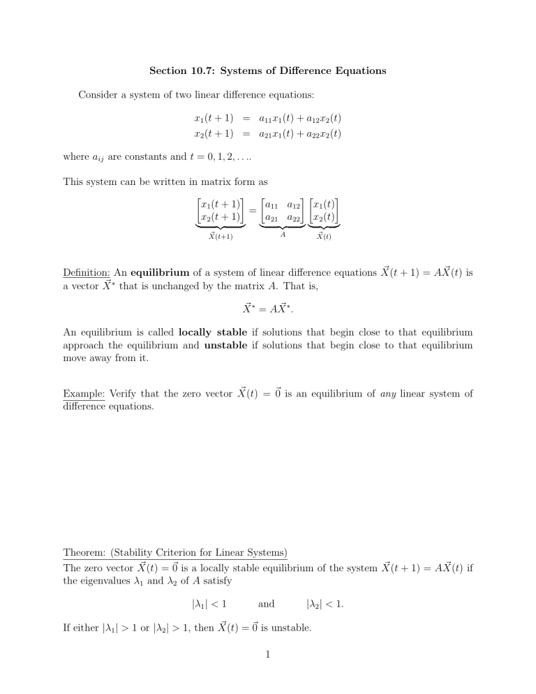
Consider a system of two linear difference equations: x
1
( t + 1) = a
11 x
1
( t ) + a
12 x
2
( t ) x
2
( t + 1) = a
21 x
1
( t ) + a
22 x
2
( t ) where a ij are constants and t = 0 , 1 , 2 , . . .
.
This system can be written in matrix form as x x
2
1
( t + 1)
( t + 1)
| {z }
~
( t +1)
= a
11 a
12 a
21 a
22 x x
2
1
( t )
( t )
| {z }
A
| {z }
~
( t )
Definition: An equilibrium of a system of linear difference equations a vector
∗ that is unchanged by the matrix A . That is,
~
( t + 1) = X ( t ) is
∗
= A ~
∗
.
An equilibrium is called locally stable if solutions that begin close to that equilibrium approach the equilibrium and unstable if solutions that begin close to that equilibrium move away from it.
Example: Verify that the zero vector difference equations.
~
( t ) = 0 is an equilibrium of any linear system of
Theorem: (Stability Criterion for Linear Systems)
The zero vector
~ the eigenvalues λ
1
( t ) = and λ
0 is a locally stable equilibrium of the system
2 of A satisfy
~
( t + 1) = X ( t ) if
| λ
2
| < 1 .
| λ
1
| < 1
If either | λ
1
| > 1 or | λ
2
| > 1, then
~
( t ) = and
1

Example: Consider the linear system x
1
( t + 1) = x
1
( t ) + 2 x
2
( t ) x
2
( t + 1) = 3 x
1
( t ) + 2 x
2
( t ) .
Write this system in matrix form and determine the stability of
~
( t ) =
Example: Consider the linear system x
1
( t + 1) = 0 .
1 x
1
( t ) + 0 .
4 x
2
( t ) x
2
( t + 1) = 0 .
1 x
1
( t ) − 0 .
2 x
2
( t ) .
Write this system in matrix form and determine the stability of
~
( t ) = 0.
2

Note: If the eigenvalues of A are complex conjugates
λ
1
= a + bi and λ
2
= a − bi, then the stability criterion can be simplified. In particular,
| λ
1
|
2
= | λ
2
|
2
= a
2
+ b
2
= ( a + bi )( a − bi ) = λ
1
λ
2
= det( A ) .
Therefore, | λ
1
| < 1 and | λ
2
| < 1 if and only if det( A ) < 1.
Example: Show that the equilibrium
~
( t ) = 0 of x
1
( t + 1) x
2
( t + 1)
=
0 .
2 0 .
3
− 0 .
5 − 0 .
4 x
1
( t ) x
2
( t ) is locally stable.
3

Nonlinear Systems
The general form of a system of two nonlinear difference equations is x
1
( t + 1) = F ( x
1
( t ) , x
2
( t )) x
2
( t + 1) = G ( x
1
( t ) , x
2
( t )) where F and G are nonlinear functions of x
1 and x
2
, and t = 0 , 1 , 2 , . . .
.
Definition: An equilibrium of a nonlinear system is a point ( x
∗
1
, x
∗
2
) such that x
∗
1 x
∗
2
= F ( x
= G ( x
∗
∗
1
1
, x
∗
, x
∗
2
2
)
) .
Example: Find all nonnegative equilibria of x
1
( t + 1) = 2 x
1
( t )[1 − x
1
( t )] x
2
( t + 1) = x
1
( t )[1 − x
2
( t )] .
4

Theorem: (Stability Criterion for Nonlinear Systems)
An equilibrium ( x
∗
1
, x
∗
2
) of the nonlinear system x
1
( t + 1) = F ( x
1
( t ) , x
2
( t )) x
2
( t + 1) = G ( x
1
( t ) , x
2
( t )) is locally stable if the eigenvalues λ
1 and λ
2 of the Jacobian matrix evaluated at ( x
∗
1
, x
∗
2
),
J ( x
∗
1
, x
∗
2
) =
F x
1
G x
1
( x
( x
∗
1
∗
1
, x
, x
∗
2
∗
2
) F x
2
) G x
2
( x
( x
∗
1
∗
1
, x
, x
∗
2
∗
2
)
) satisfy | λ
1
| < 1 and | λ
2
| < 1. If | λ
1
| > 1 or | λ
2
| > 1, then ( x
∗
1
, x
∗
2
) is unstable.
Example: Consider the nonlinear system x
1
( t + 1) = x
2
( t + 1) =
3 x
2
( t )
1 + x 2
1
( t )
2 x
1
( t )
1 + x 2
2
( t )
.
Determine the stability of the equilibrium (0 , 0).
5

Example: Show that (0 , 0) is an equilibrium of x
1
( t + 1) = ax
2
( t ) x
2
( t + 1) = 2 x
1
( t ) − cos( x
2
( t )) + 1 .
For which values of a > 0 is (0 , 0) locally stable?
6

Example: Show that (0 , 0) and ( − π, π ) are equilibria of x
1
( t + 1) = − x
2
( t ) x
2
( t + 1) = sin( x
2
( t )) − x
1
( t ) and determine their stability.
7

Example: Find all nonnegative equilibria of x
1
( t + 1) = x
2
( t ) x
2
( t + 1) =
1
2 x
1
( t ) +
2
3 x
2
( t ) − x
2
2
( t ) and determine their stability.
8

The Nicholson-Bailey Model
The Nicholson-Bailey model is a discrete-time model for host-parasitoid interactions. The model is given by the following system of nonlinear difference equations:
N t +1
P t +1
= bN t e
− aP t
= cN t
(1 − e
− aP t ) for t = 0 , 1 , 2 , . . .
.
Here, N t and P t denote the population sizes of susceptible hosts and searching adult female parasitoids at time t , respectively. The parameter b ≥ 0 is interpreted as the net growth rate for susceptible hosts. In the absence of parasitoids ( P = 0), the host population grows exponentially. The term e
− aP t denotes the fraction of hosts that are not parasitized, and so 1 − e
− aP t is the fraction of hosts that are parasitized at time t . Parasitized hosts produce parasitoids, where c ≥ 0 is the number of parasitoids produced per parasitized host.
Only nonparasitized hosts reproduce.
Numerical simulations of the Nicholson-Bailey model illustrate oscillating population sizes until either:
1. The parasitoid becomes extinct followed by exponential growth in the host population.
2. The host becomes extinct followed by extinction of the parasitoid.
Nicholson-Bailey Model
Host
Parasite
600
500
400
300
200
100
0
0 10 20 30
Time
Note: The numerical simulations of the Nicholson-Bailey model do not agree with most empirical studies.
9

Example: Find all biologically-relevant equilibria of the Nicholson-Bailey model
N t +1
P t +1
= 2 N t e
− 0 .
2 P t
= N t
(1 − e
− 0 .
2 P t ) and determine their stability.
10

The Negative Binomial Model
The negative binomial model is a modification of the Nicholson-Bailey model for which coexistence of the host and parasitoid populations is possible. The model is given by the following nonlinear system of difference equations:
N t +1
P t +1
= bN t
− k
1 + aP k
= cN t
"
1 − 1 + aP k
− k
# for t = 0 , 1 , 2 , . . .
.
Example: Find all biologically-relevant equilibria of the negative binomial model.
11

Numerical simulations of the negative binomial model illustrate dampened oscillations before stabilizing at an equilibrium ( N
∗
, P
∗
) where N
∗
> 0 and P
∗
> 0. This is known as a coexistence equilibrium since both the host and parasitoid survive.
Negative Binomial Model
400
Host
Parasite
300
200
100
0
0 10 20
Time
30 40 50
12