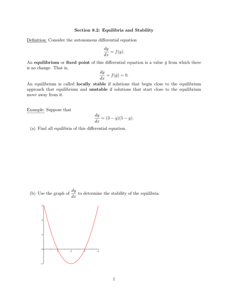
Section 8.2: Equilibria and Stability
Definition: Consider the autonomous differential equation
dy
= f (y).
dx
An equilibrium or fixed point of this differential equation is a value ȳ from which there
is no change. That is,
dy
= f (ȳ) = 0.
dx
An equilibrium is called locally stable if solutions that begin close to the equilibrium
approach that equilibrium and unstable if solutions that start close to the equilibrium
move away from it.
Example: Suppose that
dy
= (3 − y)(5 − y).
dx
(a) Find all equilibria of this differential equation.
(b) Use the graph of
dy
to determine the stability of the equilibria.
dx
1
Theorem: (Stability Criterion)
Suppose that ȳ is an equilibrium of the autonomous differential equation
dy
= f (y),
dx
where f is a differentiable function. If f 0 (ȳ) < 0, then ȳ is locally stable and if f 0 (ȳ) > 0,
then ȳ is unstable. The value f 0 (ȳ) is known as an eigenvalue.
Example: Suppose that
dy
= y(2 − y)(y − 3).
dx
(a) Find all equilibria of this differential equation.
(b) Use the graph of
dy
to determine the stability of the equilibria.
dx
(c) Compute the eigenvalues associated with each equilibrium and determine its stability.
2
Example: Suppose that a fish population evolves according to the logistic equation and
that fish are harvested at a rate proportional to the population size. If N (t) denotes the
population at time t ≥ 0, then
dN
N
= rN 1 −
− hN.
dt
K
(a) Find all biologically feasible equilibria of this differential equation.
(b) Determine the stability of each equilibrium.
(c) Find the maximal harvesting rate that maintains a positive population size.
3
Example: A tank contains 400 liters of pure water. A brine that contains 3 grams of salt per
liter enters the tank at a rate of 0.2 liters per second. The solution is kept well mixed and
drains from the tank at the same rate.
(a) Find the differential equation for the concentration, C(t), of salt in the tank at time t.
(b) Solve the differential equation and determine lim C(t).
t→∞
(c) Find all equilibria of the differential equation and determine their stability.
4
The Allee Effect
A sexually reproducing species may experience a disproportionately low recruitment rate
when the population density falls below a certain level, due to a lack of suitable mates. This
is known as an Allee effect.
Example: Let N (t) denote the size of a population at time t ≥ 0, and suppose
dN
N
= rN (N − a) 1 −
,
dt
K
where r, a, and K are positive constants and 0 < a < K. Find all equilibria of this equation
and determine their stability.
5
The Levins Model
A metapopulation is a collection of subpopulations. Each subpopulation occupies a
patch, and patches are connected via migration of individuals. In this case, we keep track of
the fraction of patches that are occupied by subpopulations.
Example: (The Levins Model) Suppose that subpopulations go extinct at a constant rate,
m > 0, which stands for mortality. Vacant patches are colonized at a rate that is proportional
to the fraction of occupied patches. The constant of proportionality is denoted by c > 0,
which stands for colonization. Let p(t) denote the fraction of occupied patches at time t ≥ 0.
Then
dp
= cp(1 − p) − mp.
dt
Find all equilibria of this equation and determine their stability.
6