Learning Compositional Sparse Models of Bimodal Percepts
Suren Kumar and Vikas Dhiman and Jason J. Corso
Computer Science and Engineering
State University of New York at Buffalo, NY
Abstract
Various perceptual domains have underlying compositional semantics that are rarely captured in current models. We suspect this is because directly learning the
compositional structure has evaded these models. Yet,
the compositional structure of a given domain can be
grounded in a separate domain thereby simplifying its
learning. To that end, we propose a new approach to
modeling bimodal percepts that explicitly relates distinct projections across each modality and then jointly
learns a bimodal sparse representation. The resulting
model enables compositionality across these distinct
projections and hence can generalize to unobserved percepts spanned by this compositional basis. For example, our model can be trained on red triangles and
blue squares; yet, implicitly will also have learned red
squares and blue triangles. The structure of the projections and hence the compositional basis is learned automatically for a given language model. To test our model,
we have acquired a new bimodal dataset comprising images and spoken utterances of colored shapes in a tabletop setup. Our experiments demonstrate the benefits of
explicitly leveraging compositionality in both quantitative and human evaluation studies.
Introduction
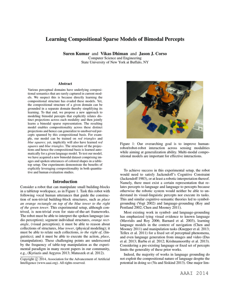
Consider a robot that can manipulate small building-blocks
in a tabletop workspace, as in Figure 1. Task this robot with
following vocal human utterances that guide the construction of non-trivial building-block structures, such as place
an orange rectangle on top of the blue tower to the right
of the green tower. This experimental setup, although contrived, is non-trivial even for state-of-the-art frameworks.
The robot must be able to interpret the spoken language (audio perception); segment individual structures, orange rectangle, (visual perception); it must be able to reason about
collections of structures, blue tower, (physical modeling); it
must be able to relate such collections, to the right of, (linguistics); and it must be able to execute the action, place,
(manipulation). These challenging points are underscored
by the frequency of table-top manipulation as the experimental paradigm in many recent papers in our community,
e.g., (Kyriazis and Argyros 2013; Matuszek et al. 2012).
c 2014, Association for the Advancement of Artificial
Copyright Intelligence (www.aaai.org). All rights reserved.
Figure 1: Our overarching goal is to improve humanrobot/robot-robot interaction across sensing modalities
while aiming at generalization ability. Multi-modal compositional models are important for effective interactions.
To achieve success in this experimental setup, the robot
would need to satisfy Jackendoff’s Cognitive Constraint
(Jackendoff 1983), or at least a robotic interpretation thereof.
Namely, there must exist a certain representation that relates percepts to language and language to percepts because
otherwise the robotic system would neither be able to understand its visual-linguistic percepts nor execute its tasks.
This and similar cognitive-semantic theories led to symbolgrounding (Vogt 2002) and language-grounding (Roy and
Pentland 2002; Chen and Mooney 2011).
Most existing work in symbol- and language-grounding
has emphasized tying visual evidence to known language
(Mavridis and Roy 2006; Barnard et al. 2003), learning
language models in the context of navigation (Chen and
Mooney 2011) and manipulation tasks (Knepper et al. 2013;
Tellex et al. 2011) for a fixed set of perceptual phenomena,
and even language generation from images and video (Das
et al. 2013; Barbu et al. 2012; Krishnamoorthy et al. 2013).
Considering a pre-existing language or fixed set of percepts
limits the generality of these prior works.
Indeed, the majority of works in language grounding do
not exploit the compositional nature of language despite the
potential in doing so (Yu and Siskind 2013). One major lim-
AAAI 2014
itation of non-compositional representation is the resulting
overwhelming learning problem. Take, the example of orange rectangle and green tower from earlier. The adjectives
orange and green are invariant to the objects rectangle and
tower. Compositional representations exploit this invariance
whereas non-compositional ones have combinatorial growth
in the size of the learning problem.
Some of the methods have enabled joint perceptuallingual adaptation to novel input (Matuszek et al. 2012;
Knepper et al. 2013) by exploiting the lingual compositionality, but none of them exploits the compositional nature of
perceptual-lingual features to introduce generative ability in
the joint model.
In this paper, we exploit the compositional nature of language for representing bimodal visual-audial percepts describing tabletop scenes similar to those in our example (Figure 1). However, we do not directly learn the compositional
structure of these percepts—attempts at doing so have met
with limited success in the literature, given the challenge of
the structure inference problem (Fidler and Leonardis 2007;
Porway, Yao, and Zhu 2008). Instead, we ground the bimodal representation in a language-based compositional
model. We fix a two-part structure wherein groupings of
visual features are mapped to audio segments. The specific mapping is not hand-tuned. Instead, it is automatically
learned from the data, and all elements of the compositional
model are learned jointly. This two-part compositional structure can take the form of adjective-noun, e.g., orange rectangle, or even noun-adjective; the method is agnostic to the
specific form of the structure. The structure is induced by
the data itself (the spoken language).
The specific representation we use is a sparse representation as it allows interpretability because the signal is represented by few bases while minimizing a goodness of fit measure. There is increasing physiological evidence that humans
use sparse coding in representation of various sensory inputs
(Barlow 1961; Lewicki 2002; Olshausen and Field 1997).
The need for sparse coding is supported by the hypothesis
of using least energy in neuron’s excitation to represent input sensory data. Furthermore, evidence suggests the multimodal sensory data is projected together on a common basis
(Knudsen and Brainard 1995), like we do in our compositional model.
We have implemented our compositional sparse model
learning for bimodal percepts in a tabletop experiment setting with real data. We observe a strong ability to learn the
model from fully observed examples, i.e., the training set
consists of all classes to be tested. More significantly, we
observe a similarly strong ability to generalize to unseen
but partially observed examples, i.e., the testing set contains
classes for whom only partial features are seen in the training set. For example, we train on blue square and red triangle and we test on blue triangle and red square. Furthermore,
this generalization ability is not observed in the state-of-theart joint baseline model we compare against.
Model
We describe our modeling approaches in this section. First,
we begin by introducing the basic bimodal paired sparse
model, which learns a sparse basis jointly over specific
visual and audial modalities. This paired sparse model is
not new (Yang et al. 2010; Wang et al. 2012; Vondrick
et al. 2013); it is the fabric of our compositional sparse
model, which we describe second. The novel compositional
sparse model jointly learns a mapping between certain feature/segment subsets, which then comprise the compositional parts to our model, and the paired sparse model for
each of them.
Paired Sparse Model
Paired sparse modeling is driven by two findings from
neurobiology (Barlow 1961; Lewicki 2002; Olshausen and
Field 1997; Knudsen and Brainard 1995): i) sparsity in representations and ii) various modality inputs are directly related. We hence use paired dictionary learning in which individual sensory data is represented by a sparse basis and
the resulting representation shares coefficients across those
bases. We are inspired by the success of paired dictionary
learning in visualizing images from features (Vondrick et al.
2013), cross-style image synthesis, image super-resolution
(Wang et al. 2012; Yang et al. 2010) and beyond.
We adapt paired dictionary learning to our problem by
learning over-complete dictionaries for sparse bases in both
the visual and audial domain while using the same coefficients across domain-bases. Following similar notation to
(Vondrick et al. 2013), let xi , yi represent visual and audio
features for the ith sample. These are related by the function mapping, xi = φ(yi ). We seek to estimate forward (φ)
and inverse (φ−1 ) mappings while representing the audio
and visual features with over-complete dictionaries (bases)
U and V , respectively, coupled by a common sparse coefficient vector α:
xi = U αi
and yi = V αi .
(1)
Sparsity in the coefficient vector is enforced by an l1 metric (Tibshirani 1996) as ||α||1 ≤ λ. This ensures that only
few bases are actively used for representing a particular input. For a given training dataset of size N , the over-complete
dictionaries U and V , and the sparse coefficient vectors {α}i
are jointly estimated by minimizing the l2 norm of the reconstruction error in both bases:
N
X
arg min
kxi − U αi k2 + kyi − V αi k2
U,V,α
s.t.
i=1
kαi k1 ≤ λ ∀i, kU k2 ≤ 1, kV k2 ≤ 1 .
(2)
Note that the bases of the over-complete dictionaries are further constrained to belong to a convex set such that individual bases have l2 norm less than or equal to unity.
The inverse mapping φ−1 for a novel sample is found by
first projecting y on the learned dictionary V and then using the obtained coefficients α∗ to compute x = U α∗ . The
process of finding these coefficients involves the following
optimization problem:
α∗ = arg min|V α − y|22 s.t kαk1 ≤ λ .
α
(3)
Similarly one can obtain the forward mapping by first projecting x on learned dictionary U to obtain α∗ and then using
Color
Red,
Blue,
...
Texture
Shape
operator. Φ is tensor of operators {Lp,q : 1 ≤ {p, q} ≤ n}
that maps audial features (xqi ) from q th audial concept to
visual features (yip ) of pth visual concept with paired dictionary learning, as described in the previous section.
We jointly solve the following optimization problem:
Circle,
Square,
...
arg
Audial Domain
Visual Domain
min
U k ,V k ,αk
s.t.
Figure 2: Mapping the physical concepts from visual domain
such as color, texture and shape to the spoken language domain
the learned dictionary V to obtain y. Thus, the estimation of
forward and inverse mapping gives one the ability to go from
audial features to visual features and vice versa. We use the
open source sparse coding package SPAMS (Mairal et al.
2010) for solving all the sparse optimization problems.
xi = Φ ? Hyi ,
(4)
where xi = [x1i , x2i , ..., xni ], yi = [yi1 , yi2 , ..., yin ] with superscript denoting the feature representation from a particular
visual or audial concept, ? denotes the element-wise product
(kxki − U k αik k2 + kyik − V k αik k2 )
i=1 k=1
kαik k1 ≤
λk ∀{i, k}, kU k k2 ≤ 1, kV k k2 ≤ 1.
(5)
The inverse mapping y 7→ x is obtained by first projecting
y on the learned basis
α∗ = arg min
αk
n
X
|V k αk − y k |22 s.t ||αk ||1 ≤ λ
(6)
k=1
and then using the linking matrix H(·). Unlike with a single
paired dictionary, there is an additional optimization problem required for forward and inverse mapping to estimate H
after estimating the Φ tensor from the learned bases,
Compositional Sparse Model
The paired model can link the two domains, but it can not
exploit the compositionality inherently present in the language. Consider, again, the utterance red square. The part
red describes the color of the object and the part square describes the shape of the object. The two parts are captured
by distinctive and co-invariant visual features. We can hence
explicitly map individual percepts between domains. Figure 2 illustrates the kind of mappings we expect to obtain
between physically grounded concepts from the visual and
audial (spoken human language) domain.
Consider n concepts, e.g., shape, from visual domain V,
which are linked to n concepts from the audial domain A.
This linking can be linearly represented by a matrix H, such
that {Vi } = H{Aj } for all {i, j} = {1, 2, ....n}. Here, we
assume that one visual concept is linked to one and only
one audial concept,Pimplying the following
two constraints
P
on the matrix: 1) j H(i, j) =
H(i,
j)
= 1 and 2)
i
each entry of the matrix can only be 1 or 0. Hence H is a
permutation matrix. Most of the counter examples of this
one-to-one mapping assumption, like ’apple’ (red circle) are
too specific to be directly grounded in just visual domain.
The linking matrix H can be time-varying due to nature of
spoken language: red rectangle and rectangle red mean the
same thing for a human but meaning different things for representation H. In this paper, we assume the audial domain
has lingual structure, i.e, it has the same ordering of concepts in spoken language. The visual feature has a natural
consistency induced by the ordering of the visual concepts.
The mapping between the ith audial and visual example
is represented by
N X
n
X
arg min
H∈H
N
X
(7)
kxi − Φ ? Hyi k2
i=1
s.t. H : H(i, j) = {0, 1},
X
H(i, j) =
j
X
H(i, j) = 1 ,
i
where H is the space of all permutation matrix.
Observe that the optimization problems in Eqs. 5 and 6
become complex as Φ and H are to be simultaneously estimated involving n2 sparse mappings and n parameters of
the permutation matrix. However, the constraints imposed
on the linking matrix H ensure that only n mappings are
used. Hence, we proceed in a sequential manner, first estimating the matrix H and then only learning the n sparse
mappings that are required. Notice also that when n = 1,
compositional sparse learning reduces to paired sparse learning.
We estimate the matrix H based on the intuition that distance in visual and in audial feature representations of the
same physically-grounded concept should co-vary. Correlation coefficients can not be directly estimated because the visual and audio features belong to different vector spaces. Instead, we estimate H based on clustering separately in each
domain and then linking clusters across domains using the
Hungarian algorithm (Kuhn 1955) and V-measure (Rosenberg and Hirschberg 2007) for cluster similarity.
Features
In this paper, we restrict our study to the concepts of color
and shape, without loss of generality. We extract color and
shape features from the visual domain and segment the audio into two parts (ideally, words) representing individual
concepts.
Visual Similar to (Matuszek et al. 2012), we first segment
the image (in HSV space). Since the shapes used in current
v1
v2
a1
0.1
0.4
a2
1
0.1
Table 1: V-measure distance matrix between the feature representation. v1 and v2 represent RGB and Fourier descriptor features, respectively, a1 and a2 represent the feature extracted from first and second audio segment.
(a) Segmented Image
(b) 2 Harmonics
(c) 10 Harmonics
Figure 3: Fourier Representation of a triangular shape with
2 and 10 fourier harmonics
work consist of basic colors, they are relatively easily segmented from the background using saturation. To represent
color, we describe each segment by its mean RGB values.
To represent the shape of each segment we opt for a global
shape descriptor based on Fourier analysis of closed contours (Kuhl and Giardina 1982).
Fourier features represent a closed contour by decomposing the contours over spectral frequency. Lower frequencies
capture the mean of shape while higher frequencies account
for subtle variations in the closed contours. The visual system of humans is found to have capabilities to form twoand three-dimensional percepts using only one-dimensional
contour information (Elder and Zucker 1993).
We extract contours of the segmented/foreground object
and use chain codes (Freeman 1974) to simplify analytical extraction of elliptic Fourier features (Kuhl and Giardina
1982). After removing the constant Fourier component, we
introduce rotational invariance by rotating of Fourier elliptical loci with respect to the major axes of the first harmonic
(Kuhl and Giardina 1982). Figure 3 shows the Fourier feature representation of a contour of a segmented triangular
shape. It can be seen that the shape is represented as a triangle even with 2 harmonics given the imperfect segmentation.
Note, the representation is invariant to position, rotation and
scale and hence the figure shows the triangle in a standardized coordinate frame.
Audio We use Mel Frequency Cepstral Coefficients
(MFCC) (Logan 2000) which are widely used in audio literature to represent audio signals. MFCC features are obtained
by dividing the audio signal into small temporal frames
and extracting cepstral features for each frame. This feature models important human perception characteristics by
ignoring phase information and modeling frequency on a
“Mel” scale (Logan 2000). Since the audio files are of different time lengths, we extract the top 20 frames with maximum spectral energy.
Experiments and Results
We perform rigorous qualitative and quantitative evaluation
to test generalization and reproduction abilities of the paired
sparse and compositional sparse models. Quantitative performance is estimated to assess reproduction ability of the
algorithm by performing 3-fold cross-validation. Qualitative
Shape\Color
Circle
HalfCircle
Rectangle
Rhombus
Square
Triangle
Trapezium
Hexagon
Total
Blue
6
6
6
10
10
8
0
0
46
Green
6
4
6
0
10
6
0
0
32
Red
2
4
6
0
10
8
10
0
40
Yellow
6
4
2
0
10
6
0
10
38
Total
20
18
20
10
40
28
10
10
Table 2: Shape and Color Exemplars in the dataset
performance is evaluated to infer the generalization capabilities of the proposed compositional sparse model and compare its performance with non-compositional paired sparse
model. For the purpose of presenting results, we only consider mapping from audio to visual in order to depict results
in the paper. However, with the model both audio to visual
and visual to audio representations can be derived.
We extract 260 dimensional audio features from selected
20 audio frames, 20 fourier harmonics, 3 dimensional color
feature and fix λ = 0.15 for all of the experiments.
Table 1 shows the evaluation of linking matrix H based
on the ground-truth data. RGB features and shape features
are denoted by v1 and v2 respectively. Audio feature a1 represent features from utterance of shape and a2 represents
features from utterance of color. This matrix gives a very
simple alignment of v1 7→ a2 and v2 7→ a1 which will be
used in compositional model.
Dataset We acquired a new dataset of shapes and colors
with 156 different examples (Table 2) of images showing a
shape captured from a camera in various rotation and translation on the tabletop. We generated machine audio that
describes the color and shape of the capture image (e.g.,
red rectangle) with random speeds. We also produced segmented audio by generating machine audio separately for
color and shape of the referred image to be used with the
compositional model.
Visualization To generate a visualization (audial-to-visual
generation), we use inverse mapping φ−1 and (H ? Φ)−1 to
generate visual features from audial features. The generated
visual feature consists of Fourier features and mean RGB intensity values. Since Fourier features are rotation and translation invariant, a close representation of original image can
not be generated. For visualizing results, we reconstruct the
50
Compositional
Paired
40
30
20
ow
yell
n
gree
red
half
circ
le
rhom
bus
trap
eziu
m
hexa
gon
trian
gle
0
blue
10
angl
e
squa
re
circ
le
40
35
30
25
20
15
10
5
0
rect
Compositional Sparse Model
Correct Retrievals
contour using Fourier features and fill the contour with predicted RGB values.
Shapes
(a) Map
(b) Color Neighbours
(c) Shape Neighbours
Paired Sparse Model
Figure 5: Comparison of correct retrievals by two different
algorithms compositional and non-compositional. Left image shows the retrieval of shape features, while right shows
that of color.
paired model can be attributed to the presence of similar examples in the training data.
(a) Map
(b) Color Neighbours
(c) Shape Neighbours
Compositional Sparse Model
Figure 4: For the audial utterance blue halfcircle, (a) generated image by mapping from audial to visual domain. (b),
(c) retrieval of color and shape neighbors by both models.
Reproduction Evaluation
For reproduction, we seek to evaluate the performance of a
robot for a theoretical command, pick a ‘red rectangle’ from
a box full of all the shapes, which is a subset of the broader
picture described in the Introduction. We perform a 3-fold
cross-validation study to assess this retrieval performance
by dividing the dataset into 3 parts, using 2 parts for training
and remaining part for testing (and then permuting the sets).
We test retrieval performance for different concepts (color
and shape) separately for paired sparse learning and compositional sparse learning. A color or shape is determined
to be correctly understood by the robot if the said color or
shape is present in top k retrieved examples. Retrieval is performed by first extracting the audial feature from the audial
stream, using the trained linking matrix to extract visual features and then picking the closest object from all the training
examples.
The closeness of a visual object to generated visual feature is measured by a distance metric in the visual feature
space. We compare the feature vectors to extract k nearest
neighbors using an l1 distance, in the appropriate concept
feature subspace. For evaluation, we set the parameter k to
be 5, which means that if there is a match in the top 5 nearest neighbors, the trial is deemed to be successful. Figure
4 shows the reproduction performance for an audial utterance blue halfcircle. It is observed that while the compositional model gets both the color and shape correct, the paired
model fails in reproducing the correct shape.
Figure 5 compares the quantitative retrieval performance
for the compositional and paired models. It is observed that
the paired model forms a good baseline for evaluating the
compositional model, which always achieves equivalent or
better performance. The reason for good performance of the
(a)
(a)
(b)
(c)
(d)
(b)
(c)
(d)
Paired Sparse Model
Figure 6: Generalization performance result depiction for
audial utterances (a) blue circle (b) green rectangle (c) red
square (d) yellow halfcircle
Generalization Evaluation
We test compositional sparse and paired sparse models with
respect to their generalization capabilities on novel samples.
Here, we test generalization across color and shape. Generalization is evaluated by generating images of a particular
color and shape whose training examples have been removed
from the dataset. For a good generalization performance, the
model must generate implicit meaning of utterances such as
green and triangle.
Figure 6 shows the pictorial results from various audio utterances from compositional sparse and paired sparse models. For the audio utterance blue circle, both models get the
right color but compositional model achieves better shape
generation which is the case for utterance green rectangle
as well. For the audial utterance red square compositional
model achieves both shape and color while the paired model
is not able to represent color. From these examples, it is
None
circle
halfcircle
hexagon
rectangle
rhombus
square
trapezium
triangle
None
Human response
(1) Comp. unbiased
0.14
0.12
0.10
0.08
0.06
0.04
0.02
0.00
0.08
0.06
0.04
Human response
Human response
(2) Paired unbiased
0.02
0.00
0.18
0.16
0.14
0.12
0.10
0.08
0.06
0.04
0.02
0.00
Human response
Human response
(3) Comp. biased
e
ow
Non
yell
red
gree
n
0.18
0.16
0.14
0.12
0.10
0.08
0.06
0.04
0.02
0.00
blue
e
ow
Non
yell
red
n
gree
blue
e
ow
Non
yell
red
gree
n
circ
halfle
hexacircle
rect gon
a
rhomngle
squa bus
trap re
e
trian zium
g
Non le
e
Machine generated shapes
Human response
0.10
0.27
0.24
0.21
0.18
0.15
0.12
0.09
0.06
0.03
0.00
Human response
0.225
0.200
0.175
0.150
0.125
0.100
0.075
0.050
0.025
0.000
circ
halfle
hexacircle
rect gon
a
rhomngle
squa bus
trap re
e
trian zium
g
Non le
e
yellow
0.12
circ
halfle
hexacircle
rect gon
a
rhomngle
squa bus
trap re
e
trian zium
g
Non le
e
red
0.16
0.14
circ
halfle
hexacircle
rect gon
a
rhomngle
squa bus
trap re
e
trian zium
g
Non le
e
green
blue
e
ow
Non
yell
red
n
gree
blue
Machine generated colors
blue
0.24
0.21
0.18
0.15
0.12
0.09
0.06
0.03
0.00
Human response
0.200
0.175
0.150
0.125
0.100
0.075
0.050
0.025
0.000
(4) Paired biased
Figure 7: Confusion matrices for generalization experiments evaluated by human subjects. Rows are for different features:
colors and shapes. Columns from left to right are four different experiments (1) Images generated by compositional model are
evaluated by humans with unbiased questions like “Describe the color and shape of this image” from fixed set of choices (2)
Paired model with unbiased questions. (3) Compositional model with biased questions like “Is the shape of generated image
same as the given example image?” 4) Paired model with biased questions.
clear that compositional model can handle generalization
both across shape and color much better compared to the
paired model. The paired sparse model—as reflected in these
results—is incompetent for this task because it does not distinguish between individual percepts.
For qualitative evaluation of generalization capabilities,
we use evaluation by human subjects. For this, we generate
two sets of images, one from the compositional model and
one from the paired model. Each set of these images is then
presented to human subjects through a web-based user interface, and the humans are asked to “Describe the color and
shape of the above image” while being presented with the
color and shape options along with “None of these” from the
training data. Note that in this experiment the human subject is not shown any samples from the training data. Hence,
we call these experiment compositional unbiased and noncompositional unbiased depending on the generating model.
In another set of experiments we bias the human subject by showing them an example image of the color and
shape for which the image has been generated. The subject
is expected to answer in “Yes” or “No” to the question: “Is
the color (shape) of the above image same as the example
image?” Whenever the subject says “Yes”, we take the response as the expected color/shape; for “No” we assume
“None of these” option.
Figure 7 shows the human qualitative performance metrics for this test. It is observed that color generalizes almost
perfectly using our proposed compositional sparse model
while the paired sparse model gives poor performance in
both biased and unbiased human evaluation. On the generalization of shape, the compositional model again achieves
much better performance over the baseline paired model in
both biased and unbiased experiments. Using the internal semantics of humans, it is observed that halfcircle is frequently
represented as rectangle or trapezium for the compositional
model. It is likely because of the shape feature with invariance whose closed contour representation is not enough to
distinguish perceptually similar shapes. Furthermore, triangle is often mistaken as trapezium which can be explained by
a similar starting sound. It is seen that biased results give better performance denoting improved assessment after recalibration of human semantics to current experimental shapes.
Conclusion
We propose a novel model representing bimodal percepts
that exploits the compositional structure of language. Our
compositional sparse learning approach jointly learns the
over-complete dictionaries, sparse bases, and cross-modal
linking matrix. In contrast to prior work in bimodal modeling which is primarily discriminative in nature, e.g., (Roy
and Pentland 2002; Roller and Schulte im Walde 2013), our
compositional sparse learning approach is generative and
hence transparent. We demonstrate the effectiveness of sparsity and compositionality by both qualitative and quantitative evaluations.
References
Barbu, A.; Bridge, A.; Burchill, Z.; Coroian, D.; Dickinson,
S.; Fidler, S.; Michaux, A.; Mussman, S.; Narayanaswamy,
S.; Salvi, D.; Schmidt, L.; Shangguan, J.; Siskind, J. M.;
Waggoner, J.; Wang, S.; Wei, J.; Yin, Y.; and Zhang, Z. 2012.
Video in sentences out. In UAI.
Barlow, H. B. 1961. Possible principles underlying the
transformation of sensory messages. Sensory communication 217–234.
Barnard, K.; Duygulu, P.; Forsyth, D.; de Frietas, N.; Blei,
D. M.; and Jordan, M. I. 2003. Matching words and pictures.
Journal of Machine Learning Research 3:1107–1135.
Chen, D. L., and Mooney, R. J. 2011. Learning to interpret
natural language navigation instructions from observations.
In AAAI.
Das, P.; Xu, C.; Doell, R. F.; and Corso, J. J. 2013. A
thousand frames in just a few words: Lingual description of
videos through latent topics and sparse object stitching. In
CVPR.
Elder, J., and Zucker, S. 1993. The effect of contour closure on the rapid discrimination of two-dimensional shapes.
Vision research 33(7):981–991.
Fidler, S., and Leonardis, A. 2007. Towards scalable representations of object categories: Learning a hierarchy of
parts. In CVPR. IEEE.
Freeman, H. 1974. Computer processing of line-drawing
images. ACM Computing Surveys (CSUR) 6(1):57–97.
Jackendoff, R. 1983. Semantics and Cognition. MIT Press.
Knepper, R. A.; Tellex, S.; Li, A.; Roy, N.; and Rus, D. 2013.
Single assembly robot in search of human partner: versatile grounded language generation. In HRI, 167–168. IEEE
Press.
Knudsen, E., and Brainard, M. 1995. Creating a unified representation of visual and auditory space in the brain. Annual
review of neuroscience 18(1):19–43.
Krishnamoorthy, N.; Malkarnenkar, G.; Mooney, R. J.;
Saenko, K.; and Guadarrama, S. 2013. Generating naturallanguage video descriptions using text-mined knowledge. In
AAAI.
Kuhl, F. P., and Giardina, C. R. 1982. Elliptic fourier features of a closed contour. Computer graphics and image
processing 18(3):236–258.
Kuhn, H. W. 1955. The hungarian method for the assignment problem. Naval research logistics quarterly 2(1-2):83–
97.
Kyriazis, N., and Argyros, A. 2013. Physically plausible 3D
scene tracking: The single actor hypothesis. In CVPR.
Lewicki, M. S. 2002. Efficient coding of natural sounds.
Nature neuroscience 5(4):356–363.
Logan, B. 2000. Mel frequency cepstral coefficients for
music modeling. In ISMIR.
Mairal, J.; Bach, F.; Ponce, J.; and Sapiro, G. 2010. Online learning for matrix factorization and sparse coding. The
Journal of Machine Learning Research 11:19–60.
Matuszek, C.; Fitzgerald, N.; Zettlemoyer, L.; Bo, L.; and
Fox, D. 2012. A joint model of language and perception for
grounded attribute learning. In ICML.
Mavridis, N., and Roy, D. 2006. Grounded situation models
for robots: Where words and percepts meet. In IROS.
Olshausen, B. A., and Field, D. J. 1997. Sparse coding
with an overcomplete basis set: A strategy employed by v1?
Vision research 37(23):3311–3325.
Porway, J.; Yao, B.; and Zhu, S. C. 2008. Learning compositional models for object categories from small sample sets.
Object categorization: computer and human vision perspectives.
Roller, S., and Schulte im Walde, S. 2013. A multimodal
LDA model integrating textual, cognitive and visual modalities. In EMNLP, 1146–1157.
Rosenberg, A., and Hirschberg, J. 2007. V-measure: A conditional entropy-based external cluster evaluation measure.
In EMNLP-CoNLL, volume 7, 410–420.
Roy, D. K., and Pentland, A. P. 2002. Learning words from
sights and sounds: A computational model. Cognitive science 26(1):113–146.
Tellex, S.; Kollar, T.; Dickerson, S.; Walter, M. R.; Banerjee,
A. G.; Teller, S.; and Roy, N. 2011. Understanding natural
language commands for robotic navigation and mobile manipulation. Proc. AAAI.
Tibshirani, R. 1996. Regression shrinkage and selection via
the lasso. Journal of the Royal Statistical Society. Series B
(Methodological) 267–288.
Vogt, P. 2002. The physical symbol grounding problem.
Cognitive Systems Research 3(3):429–457.
Vondrick, C.; Khosla, A.; Malisiewicz, T.; and Torralba, A.
2013. HOG-gles: Visualizing object detection features. In
ICCV.
Wang, S.; Zhang, L.; Liang, Y.; and Pan, Q. 2012.
Semi-coupled dictionary learning with applications to image super-resolution and photo-sketch synthesis. In CVPR,
2216–2223. IEEE.
Yang, J.; Wright, J.; Huang, T. S.; and Ma, Y. 2010. Image
super-resolution via sparse representation. Image Processing, IEEE Transactions on 19(11):2861–2873.
Yu, H., and Siskind, J. M. 2013. Grounded language learning from videos described With sentences. In ACL.