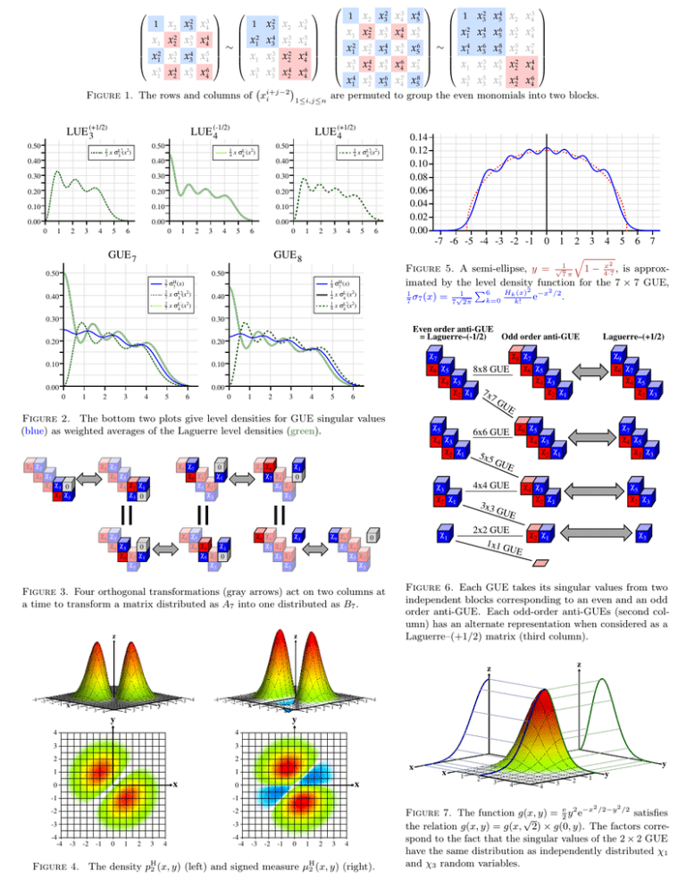

1
2
3
x

3
4
x

2
3
1
x
3
4
x


x x
2
2

 

 x x2 x3 x4   x2 x4 x3 x5 
 1 2 3 4   1 3 2 4 

∼

 x2 x3 x4 x5   x x3 x2 x4 
 1 2 3 4   1 3 2 4 
x13 x24 x35 x46
(+1/2)
0.50
1
3
1≤i,j≤n
(-1/2)
0.50
+
1
4
0.50
-
x σL4 (x2)
0.40
0.40
0.30
0.30
0.30
0.20
0.20
0.20
0.10
0.10
0.10
0.00
0
1
2
3
4
5
1
4
+
x σL4 (x2)
0.00
6
0
1
2
3
4
x32 x54 x2 x43

x13 x35 x57 x24 x46
are permuted to group the even monomials into two blocks.
LUE 4
0.40
0.00
1
(+1/2)
LUE 4
x σL3 (x2)

x14 x25 x36 x47 x58
i+j−2
LUE 3


 

 x x2 x3 x4 x5   x2 x4 x6 x3 x5 
 1 2 3 4 5   1 3 5 2 4 
 2 3 4 5 6   4 6 8 5 7 
 x1 x2 x3 x4 x5  ∼  x1 x3 x5 x2 x4 

 

 x3 x4 x5 x6 x7   x x3 x5 x2 x4 
 1 2 3 4 5   1 3 5 2 4 
x13 x35 x24 x46
Figure 1. The rows and columns of xi
x2 x32 x43 x54
1
5
6
0
1
2
3
4
5
6
0.14
0.12
0.10
0.08
0.06
0.04
0.02
0.00
-7 -6 -5 -4 -3 -2 -1
GUE 7
GUE 8
0.50
0.50
2
7
2
7
2
7
0.40
1
4
1
4
1
4
σH
(x)
7
+
x σL3 (x2)
0.40
-
x σL4 (x2)
0.30
0.30
0.20
0.20
0.10
0.10
0.00
σH
(x)
7
-
x σL4 (x2)
+
x σL4 (x2)
1
2
3
4
5
6
0
1
2
3
4
5
1
2
3
4
5
6
7
q
x2
Figure 5. A semi-ellipse, y = √17 π 1 − 4·7
, is approximated by the level density function for the 7 × 7 GUE,
P
(x)2 −x2 /2
1
σ (x) = 7√12π 6k=0 Hkk!
e
.
7 7
Even order anti-GUE
= Laguerre–(-1/2)
Odd order anti-GUE
Laguerre–(+1/2)
χ7
χ8 χ7
χ6 χ5
8x8 GUE χ6 χ5
χ4 χ3
χ4 χ3
χ2 χ1 7x
χ2 χ1
χ9
χ6 χ7
χ4 χ5
χ2 χ3
0.00
0
0
7G
6
UE
Figure 2. The bottom two plots give level densities for GUE singular values
(blue) as weighted averages of the Laguerre level densities (green).
χ8 χ7
χ6 χ5
χ4 χ3 0
χ2 χ1
χ8 χ7
χ6 χ5
χ4 χ2 χ1
χ3 0
χ8 χ7
0
χ6 χ4
χ1
χ5 χ2
χ3
χ8 χ7
χ6 χ5
0
χ4 χ2 χ1
χ3
χ5
χ4 χ3
χ2 χ1
4x4 GUE
χ3
χ2 χ1
χ8 χ6
χ1
χ7 χ4
χ5 χ2
χ3
z
3x3
χ7
χ4 χ5
χ2 χ3
χ4 χ3
χ2 χ1
χ5
χ2 χ3
GUE
2x2 GUE
χ2 χ1
1x1 G
UE
χ1
χ9 χ6
0
χ7 χ4
χ5 χ2
χ3
Figure 3. Four orthogonal transformations (gray arrows) act on two columns at
a time to transform a matrix distributed as A7 into one distributed as B7 .
z
5x5
G
χ6 χ5
χ4 χ3
χ2 χ1
UE
χ8 χ6
χ1
χ7 χ4
0
χ5 χ2
χ3
χ8 χ7
χ6 χ4
χ1
χ5 χ2 0
χ3
6x6 GUE
χ3
Figure 6. Each GUE takes its singular values from two
independent blocks corresponding to an even and an odd
order anti-GUE. Each odd-order anti-GUEs (second column) has an alternate representation when considered as a
Laguerre–(+1/2) matrix (third column).
z
z
-4 -3
-2 -1
x
1
2
3
4
4
2
3
1
y
-3 -4
-1 -2
-4 -3
-2 -1
x
1
2
3
y
4
3
3
2
2
1
1
0
x
-1
-2
-2
-3
-3
-2
-1
0
2
3
1
y
-3 -4
-1 -2
1
2
3
4
-4
-4
x
x
x
0
-1
-3
4
y
4
-4
-4
4
x
y
y
1
2
3
4
4
3
2
y
1
2
-3
-2
-1
0
1
2
3
4
H
Figure 4. The density pH
2 (x, y) (left) and signed measure µ2 (x, y) (right).
2
Figure 7. The function g(x, y) = 2e y 2 e−x /2−y /2 satisfies
√
the relation g(x, y) = g(x, 2) × g(0, y). The factors correspond to the fact that the singular values of the 2 × 2 GUE
have the same distribution as independently distributed χ1
and χ3 random variables.