Math 323
Change of Basis Notation
October 27, 2013
Since the notation in the book is not entirely the same (or as useful) as what we have done
in class, I’ve summarized the important things below.
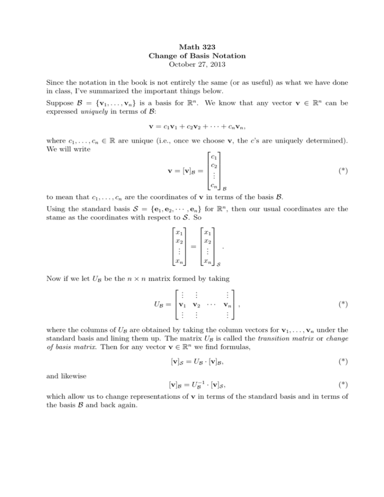
Suppose B = {v1 , . . . , vn } is a basis for Rn . We know that any vector v ∈ Rn can be
expressed uniquely in terms of B:
v = c1 v 1 + c2 v 2 + · · · + cn v n ,
where c1 , . . . , cn ∈ R are unique (i.e., once we choose v, the c’s are uniquely determined).
We will write
 
c1
 c2 
 
v = [v]B =  .. 
(*)
.
cn B
to mean that c1 , . . . , cn are the coordinates of v in terms of the basis B.
Using the standard basis S = {e1 , e2 , · · · , en } for Rn , then our usual coordinates are the
stame as the coordinates with respect to S. So
   
x1
x1
 x2   x2 
   
 ..  =  ..  .
. .
xn
xn S
Now if we let UB be the n × n matrix formed by taking
.
..
.. 
..
.
.


UB = v1 v2 · · · vn  ,
..
..
..
.
.
.
(*)
where the columns of UB are obtained by taking the column vectors for v1 , . . . , vn under the
standard basis and lining them up. The matrix UB is called the transition matrix or change
of basis matrix. Then for any vector v ∈ Rn we find formulas,
[v]S = UB · [v]B ,
(*)
[v]B = UB−1 · [v]S ,
(*)
and likewise
which allow us to change representations of v in terms of the standard basis and in terms of
the basis B and back again.
If A = {u1 , u2 , . . . , un } is another basis for Rn , then we can interchange between B-basis
representations and A-representations: for any v ∈ Rn ,
[v]A = UA−1 UB · [v]B
and likewise
[v]B = UB−1 UA · [v]B .
Now suppose that L : Rn → Rm is a linear transformation. Suppose that B = {v1 , v2 , . . . , vn }
is a basis for Rn and C = {w1 , w2 , . . . , wm } is a basis for Rm . Then there is an m × n matrix
[L]CB so that
∀x ∈ Rn .
[L(x)]C = [L]CB [x]B ,
In fact,
..
..
.
.

[L]CB = [L(v1 )]C [L(v2 )]C · · ·
..
..
.
.


..
.

[L(vn )]C  .
..
.
(*)
To think about what this means: [L]CB takes as input vectors in coordinates with respect to
B, applies L to them, and then leaves as output vectors in coordinates with respect to C.
Example 1: We know that any linear transformation L : Rn → Rm is represented by an
m × n matrix A:
L(x) = Ax,
∀x ∈ Rn ,
and
..
..
.
.

A = L(e1 ) L(e2 ) · · ·
..
..
.
.

.. 
.

L(en ) .
..
.
Everything here is done in terms of the standard basis. So what we have is
 .
..
.. 
..
.
.


Sm
[L]Sn = A = L(e1 ) L(e2 ) · · · L(en ) .
..
..
..
.
.
.
(*)
Example 2: Let I : Rn → Rn be the identity transformation,
I(x) = x,
∀x ∈ Rn .
We can represent I in terms of a basis B = {v1 , v2 , . . . , vn }, and we find
.
..
.. 
..
.
.


S
[I]B = UB = v1 v2 · · · vn  ,
..
..
..
.
.
.
(*)
where S is the standard basis on Rn . Likewise,
[I]BS = ([I]SB )−1 = UB−1 .
(*)
If L : Rn → Rn is a linear transformation, the representation of L in terms of the basis B is
[L]BB = [I]BS · [L]SS · [I]SB
= ([I]SB )−1 · [L]SS · [I]SB .
(*)
For any linear transformation, L : Rn → Rm , we can find [L]SSm
from Example 1 above. If B
n
n
m
is any basis of R and C is any basis of R ,
· [I]SBn .
[L]CB = [I]CSm · [L]SSm
n
(*)
Example 3: Let L : R3 → R3 be given by
  
 
x1
1 2 3 x1
L x2  =  0 1 0 x2  .
x3
−1 0 9 x3
nh −1 i h i h io
nh 0 i h i h io
2
4
0
1
0
1 , 1
1
Let B =
, 0 , 1 , and let C =
,
. Let S be the standard basis
−1
0
1
2
3
on R3 . Things you should check:


−1 2 4
[I]SB =  1 0 1 ;
0 1 2
and


1 2 3
[L]SS =  0 1 0 ;
−1 0 9
5


1
3
9
[I]CB =  2 −2 −3 .
−1 2
4


3
7 −3
[L]CS = −1 −1 −3 .
1
2
3
and
[L]CB = ??
[L]BC = ??