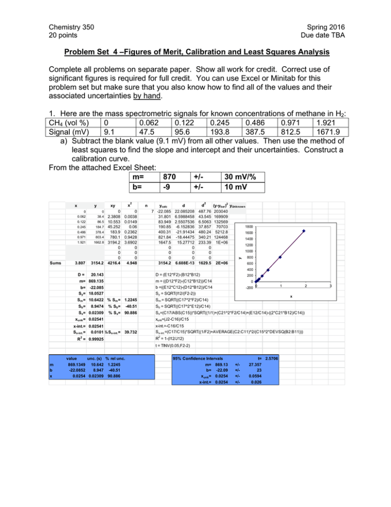
Chemistry 350
20 points
Spring 2016
Due date TBA
Problem Set 4 –Figures of Merit, Calibration and Least Squares Analysis
Complete all problems on separate paper. Show all work for credit. Correct use of
significant figures is required for full credit. You can use Excel or Minitab for this
problem set but make sure that you also know how to find all of the values and their
associated uncertainties by hand.
1. Here are the mass spectrometric signals for known concentrations of methane in H2:
CH4 (vol %)
0
0.062
0.122
0.245
0.486
0.971
1.921
Signal (mV)
9.1
47.5
95.6
193.8
387.5
812.5
1671.9
a) Subtract the blank value (9.1 mV) from all other values. Then use the method of
least squares to find the slope and intercept and their uncertainties. Construct a
calibration curve.
From the attached Excel Sheet:
m=
870
+/30 mV/%
b=
-9
+/10 mV
Sums
y
x
xy
0
0
0.062
38.4
0.122
86.5
0.245
184.7
0.486
378.4
0.971
803.4
1.921
1662.8
3.807
3154.2
D=
20.143
0
2.3808
10.553
45.252
183.9
780.1
3194.2
0
0
0
4216.4
2
0
0.0038
0.0149
0.06
0.2362
0.9428
3.6902
0
0
0
4.948
n
ycalc
d
7 -22.085 22.085208
31.801 6.5988458
83.949 2.5507536
190.85 -6.152836
400.31 -21.91434
821.84 -18.44475
1647.5
15.27712
0
0
0
0
0
0
3154.2 6.608E-13
d
2
487.76
43.545
6.5063
37.857
480.24
340.21
233.39
0
0
0
1629.5
2
(y-ybar ) yUnknow n
203040
169909
132569
1800
70703
5212.8
1600
124468
1400
1E+06
1200
1000
y
x
2E+06
800
600
400
D = (E12*F2)-(B12*B12)
200
m= 869.135
m = ((D12*F2)-(C12*B12))/C14
0
b= -22.085
Sy= 18.0527
b =((E12*C12)-(D12*B12))/C14
Sy = SQRT(I12/(F2-2))
-200
Sm = 10.6422 % Sm = 1.2245
Sm = SQRT((C17^2*F2)/C14)
Sb=
Sb = SQRT((C17^2*E12)/C14)
8.9474
Sx= 0.02309
% S b=
-40.51
% Sx= 90.886
0
1
x
Sx=(C17/ABS(C15))*SQRT((1/1)+(C21^2*F2/C14)+(E12/C14)-((2*C21*B12)/C14))
xunk=(J2-C16)/C15
xunk = 0.02541
x-int.= 0.02541
Sx-int.= 0.0101 % Sx-int.= 39.732
x-int.=-C16/C15
Sx-int.=(C17/C15)*SQRT((1/F2)+AVERAGE(C2:C11)^2/(C15^2*DEVSQ(B2:B11)))
2
2
R = 1-(I12/J12)
R = 0.99925
t = TINV(0.05,F2-2)
value
m
b
x
unc. (s) % rel unc.
869.1349 10.642
-22.0852
8.947
0.0254 0.02309
2
1.2245
-40.51
90.886
95% Confidence Intervals
m= 869.13
b= -22.09
xunk = 0.0254
x-int.= 0.0254
t= 2.5706
+/+/+/+/-
27.357
23
0.0594
0.026
3
Chemistry 260
Chapter 1 – Introduction
2
b) Replicate measurements of an unknown gave 152.1, 154.9, 153.9, and 155.1 mV.
Determine the concentration of the unknown and its uncertainty. Determine the
95% confidence interval for the unknown.
To use our calibration curve, we must subtract the blank signal off first.
Raw
Signal
152.1
154.9
153.9
155.1
Corrected
Signal
143.0
145.8
144.8
146
Vol %
0.189942
0.193164
0.192013
0.193394
Mean
Stdev
t
CI
0.192128 %
0.001578 %
3.182446
0.00251 %
So the confidence interval is 0.192 ±0.003 %
c) A blank gave 8.2, 9.4, 10.6, 8.4, 9.6, 7.4 and 7.8 mV when measured multiple
times. Determine the limit of detection at the 99% confidence level for the
procedure.
From these values, the standard deviation of the blank signal is 8.77 mV with a
standard deviation of 1.13 mV. Therefore our signal at the detection limit is:
8.77mV + 3(1.13) = 12.17 mV
Again, to use the calibration relationship, we need to subtract the blank signal (9.1 mV)
from this value: 12.17-9.1 = 3.07 mV.
Now we convert this to a concentration using the calibration relationship to find the
LOD
LOD = (3.07-(-20))mV/(870 mV/%) = 0.027%
Chemistry 260
Chapter 1 – Introduction
3
2. Pure water containing no arsenic was spiked with 0.40 g arsenate/L. Seven
replicate determinations gave 0.39, 0.40, 0.38, 0.41, 0.36, 0.35, and 0.39 g/L
arsenic. Find the mean percent recovery of the spike and the detection limit for the
method.
%recovery
g
arsenate/L
0.39
97.5
0.4
100
0.38
95
0.41
102.5
0.36
90
0.35
87.5
0.39
97.5
Mean 0.382857 95.71429
Stdev 0.021381 5.345225
LOD
0.064143
The percent recovery is 100%x(Cspiked sample – Cunspiked sample)/Cadded. In our case
Cunspiked sample = 0 g arsenate/L and Cadded = 0.40 g arsenate/L
To find the LOD, we need the standard deviation of the measurements. Since they are
already in concentration units and since we assume that a 0 g arsenate/L sample
would give 0 concentration, our LOD is simply 3 times the standard deviaton of the
sample concentrations. LOD = 3(0.021381 g arsenate/L) = 0.06 g arsenate/L
3. An unknown sample of Cu2+ gave an absorbance of 0.262 in an atomic absorption
analysis. Then 1.00 mL of a solution containing 100.0 ppm (i.e. g/mL) Cu2+ was
mixed with 95.0 mL of the unknown and the mixture was diluted to 100.0 mL in a
volumetric flask with DI water. The absorbance of the new solution was 0.500.
a. Denoting the initial, unknown concentration as [Cu2+]i, write an expression
for the final concentration, [Cu2+]f, after dilution. Units of concentration
are ppm.
[Cu2+]f = (95 mL/100 mL)[Cu2+]i
b. In a similar manner, write the final concentration of added standard Cu2+,
designated as [S]f
[S]f = (1 mL/100 mL)[S]I = (1/100)x100.0 ppm = 1.000 ppm
c. Find [Cu2+]I in the unknown.
0.262
0.500 1.000 0.95
After some algebra, [Cu2+]i = 1.04 ppm
Chemistry 260
Chapter 1 – Introduction
4
4. A constant volume standard addition experiment is performed. Five flasks
containing 25.00 mL of a serum with unknown concentration of Na+ are labeled 1-5.
Into each, varying volumes (see below) of 2.640 M NaCl standard is added. Each
flask is then diluted to 50.00 mL.
Flask
1
2
3
4
5
Volume of standard added (mL)
0
1.000
2.000
3.000
4.000
Na+ atomic emission signal (mV)
3.13
5.40
7.89
10.30
12.48
a. Use Excel or Minitab to prepare a standard addition graph and find the
concentration of Na+ in the serum.
volume concentration
added
added
(mL)
(M)
0
0
1
0.0528
2
0.1056
3
0.1584
4
0.2112
signal
3.13
5.4
7.89
10.3
12.48
From a least-squares analysis, we find the equation of our line to be:
Signal in mV = 44.697mV/M(concentration) + 3.12mV
Solving for the x-intercept (y=0)
0 mV = 44.697mV/M(concentration) + 3.12mV
Concentration = -(-3.12mV/(44.697mV/M)) = 0.0698 M
Since this was in the solution that was measured, we must account for dilution to
determine the original concentration: 0.0698M(50.00mL/25.00mL) = 0.1396M
b. Determine the uncertainty in the result.
Here we need the sx-intercept, which from our least squared analysis is 0.00235 or
3.367%. So our uncertainty in the final concentration is 0.003367(0.1396M) = 0.0047M
So our final result would be 0.140±0.005M, where we have estimated our uncertainty
using the standard deviation. We could convert that to a confidence interval by
multiplying by the appropriate t-value (t=3.1824 for 3 degrees of freedom)