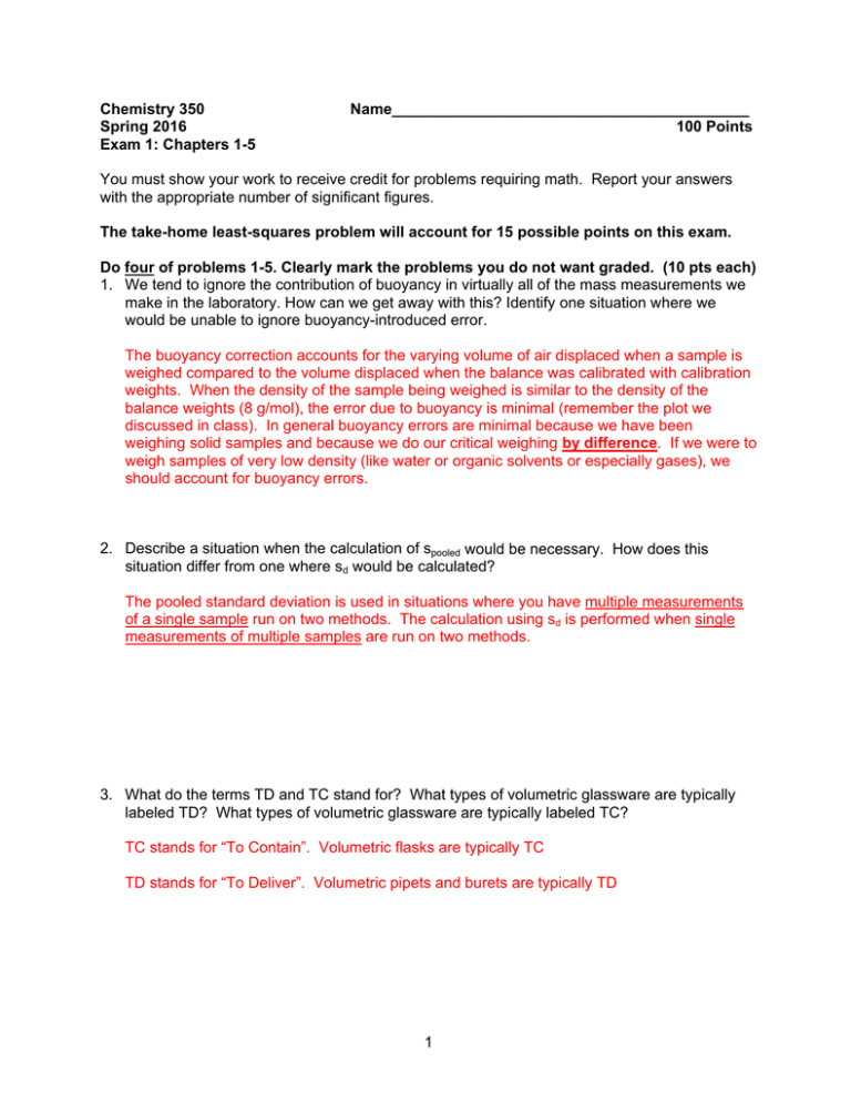
Chemistry 350
Spring 2016
Exam 1: Chapters 1-5
Name__________________________________________
100 Points
You must show your work to receive credit for problems requiring math. Report your answers
with the appropriate number of significant figures.
The take-home least-squares problem will account for 15 possible points on this exam.
Do four of problems 1-5. Clearly mark the problems you do not want graded. (10 pts each)
1. We tend to ignore the contribution of buoyancy in virtually all of the mass measurements we
make in the laboratory. How can we get away with this? Identify one situation where we
would be unable to ignore buoyancy-introduced error.
The buoyancy correction accounts for the varying volume of air displaced when a sample is
weighed compared to the volume displaced when the balance was calibrated with calibration
weights. When the density of the sample being weighed is similar to the density of the
balance weights (8 g/mol), the error due to buoyancy is minimal (remember the plot we
discussed in class). In general buoyancy errors are minimal because we have been
weighing solid samples and because we do our critical weighing by difference. If we were to
weigh samples of very low density (like water or organic solvents or especially gases), we
should account for buoyancy errors.
2. Describe a situation when the calculation of spooled would be necessary. How does this
situation differ from one where sd would be calculated?
The pooled standard deviation is used in situations where you have multiple measurements
of a single sample run on two methods. The calculation using sd is performed when single
measurements of multiple samples are run on two methods.
3. What do the terms TD and TC stand for? What types of volumetric glassware are typically
labeled TD? What types of volumetric glassware are typically labeled TC?
TC stands for “To Contain”. Volumetric flasks are typically TC
TD stands for “To Deliver”. Volumetric pipets and burets are typically TD
1
4. Whenever we use a confidence interval to represent the proximity of our results to the “true”
value, we are forced to make an important assumption. What assumption must be made to
use such a statistical analysis to reflect the accuracy of a measurement? Why is this
assumption necessary?
The confidence interval also allows us to make some inferences about the accuracy of a method
by taking the fact that we have a small data set into account; assuming only random errors are
impacting our measurement. Therefore, we must rely on good experimental design to remove
systematic errors to make an evaluation using the confidence interval reasonable.
5. Outline the process that would typically be used in lab to perform a standard additions
experiment. (hint: you will need more than two solutions)






Prepare a series of solutions, each containing the same amount of your unknown solution
and "spiked" with a different (and known) concentration of analyte (including "0")
Perform analysis using each solution
Plot signal vs. added analyte concentration
Calculate least-squares line
Extrapolate the line to the x-intercept. The unknown concentration in the measured
solution corresponds to the value at the x-intercept.
Account for any dilutions to determine the analyte concentration in your original unknown
solution.
2
Do three of problems 6-9. Clearly mark the problems you do not want graded. (15 pts
each)
6. A solution was prepared by dissolving 1.975 grams of a solid sample containing an unknown
amount of mercury in a total of 100.00 mL of solution, which was labeled solution A. Before
analysis, 5.00 mL of solution A was pipetted into a 100.00 mL volumetric flask, mixed and
diluted to the mark to form solution B. Then 10.00 mL of solution B was pipetted into a
25.00 mL volumetric flask, mixed and diluted to the mark to make solution C. Analysis of
solution C determined that it had a mercury concentration of 12.6 ppm. What was the
percent mercury by mass in the original solid sample? You may assume a density of
1.00 g/mL for all solutions.
It is useful to think of ppm Hg as g Hg/mL solution (or mg Hg/L solution). This isn’t
essential, but it makes the dimensional analysis a little more streamlined.
We need to first account for each of the dilutions to determine the concentration of mercury in
the original solution:
12.6 g Hg x 25.00 mL C x 100.00 mL B = 630 g Hg
mL C
10.00 mL B
5.00 mL A
mL A
Now we can determine the mass of Hg in solution A:
-6
630 g Hg x 100.00 mL A x 10 g Hg = 0.0630 g Hg
mL A
g Hg
Finally, determine %Hg:
0.0630 g Hg
x 100 % = 3.19 % Hg
1.975 g sample
3
7. Low concentrations of thallium near the detection limit gave the following dimensionless
instrument readings: 211.3, 178.9, 168.3, 180.3, 225.3, 166.1, 229.1, 207.7, 140.7, and
211.5. Ten blanks had a mean reading of 43.9. The slope of the calibration curve is
1.10×109 M–1. Estimate the detection limit for thallium.
The average of the measurements is: 191.92
The standard deviation is: 29.17. We assume the standard deviation of the blanks is the same
So, the signal at the detection limit is:
yLOD = yblank + 3sblank
yLOD = 43.9 + 3(29.17) = 131.4
We can use the slope to convert this to a concentration:
LOD = 131.4/(1.10x109 M-1) = 1.19x10-7 M
4
8. A Standard Reference Material is certified to contain 45.4 ppm of an organic contaminant in
soil. You analyze this material to characterize a new method you are developing. Your
analysis gives values of 47.8, 47.4, 45.6, 48.4, and 47.2 ppm. Evaluate the results for
suspect data and determine whether your results indicate the presence of systematic error in
your method at the 95% confidence level. Justify your answer.
Based on the full dataset, the mean is 47.2 ppm, and s = 0.97 ppm
With all of the other data bunched around 47 and 48 ppm, the point at 45.6 ppm should look
a little odd and worthy of a Q-test. Q for 5 observations is 0.64
47.2-45.6
=
1.6
=
0.64 is not > 0.64 so retain 45.6
48.1-45.6
2.5
If you choose to do the Grubb’s test, G for 5 observations is 1.672:
47.2-45.6
=
1.6
= 1.649 < 1.672 so retain 45.6
1.19
0.97
To determine whether systematic error is indicated, determine if the “true value” falls within
the confidence interval. (using the 95% confidence level). For 4 degrees of freedom and
95%, ttable = 2.776
2.776  0.97
ts
CI  47.2 
 47.2 
 47.2  1.20
n
5
So, the confidence range is 47 ± 1 ppm, which does not include the true value, therefore,
there seems to be an indication of systematic error (at least a 5% chance).
You could also calculate a t value to compare to the tabulated t:
t calc 
true value  x
s
n
45.4  47.2
0.97
5  4.15
Since tcalc > ttable there is a statistically significant difference.
5
9. Acid solutions can be standardized using primary standard sodium carbonate, much like
base solutions can be standardized using pure KHP as we did in lab. Below is data from a
titration of a sodium carbonate sample with a solution of hydrochloric acid of unknown
concentration. In this titration, approximately 25 mL of distilled water was used to dissolve
the sodium carbonate that was dispensed from the weighing bottle into an Erlenmeyer flask.
What is the molarity of the hydrochloric acid solution with its absolute uncertainty?
Initial mass of weighing bottle and sodium carbonate
Final mass of weighing bottle after sample was removed
Initial buret reading
Final buret reading
Molar mass of sodium carbonate
32.13840.0002 g
30.96150.0002 g
2.380.02 mL
39.540.02 mL
105.98850.0002 g/mol
Our reaction of interest is:
Na2CO3 + 2HCl → H2CO3 + 2NaCl
Our general calculation is:
(mem)g Na2CO3 x
x
2 mol HCl
x
1
= [HCl]
1 mol Na2CO3
1
mol
Na
CO
(MMeMM)g Na2CO3
(Vev)L solution
2
3
We are given the molar mass and its uncertainty, but need to calculate the mass and
uncertainty of Na2CO3 and volume and uncertainty of HCl solution.
Mass Na2CO3 = 32.1384-30.9615 g = 1.1769 g
Uncertainty in mass:
em 
0.0002g2  0.0002g2
 0.00028 g
Volume HCl = 39.54-2.38 mL = 37.16 mL
Uncertainty in volume:
ev 
0.02 mL 2  0.02 mL 2
 0.028 mL
Now we can insert these values into our calculation
(1.17690.00028)g x
Na2CO3
1 mol Na2CO3
x 2 mol HCl x
1
(105.98850.0002)g
Na2CO3
1 mol
Na2CO3
(37.160.028)x10-3 L
solution
2
2
2
= (0.5976e[]) M
HCl
 0.00028 g   0.028 mL   0.0002 g / mol 
  
  
  0.5976 M0.00079  0.00047 M
e[]  0.5976 M 
 1.1769 g   37.16 mL   105.9885 g / mol 
So, the HCl concentration is 0.5976  0.0005 M
6
Possibly Useful Information

d 
m' 1  a 
d
w
m 
 da 
1 

d 

Density of balance weights = 8.0 g/ml
ts
x 
y
n
eC  e  e
2
A
t calculated 
Density of air = 0.012 g/ml
s
x1  x 2
s pooled
n
n1n 2
n1  n 2
spooled 
sy
m
sy 
s 2y  n
2
sm 
n 1
s12 n1  1  s22 n2  1
n1  n2  2


 di  d
i
2
n 1
 di  d
n2
2

2
 di
n2
2
2
2 s y  xi
sb 
D
D
Fcalculated 
yLOD = yblank + 3s
Q calculated 
2
i
sd 
1 1
( y  y )2
 
k n m 2  x i  x 2
2
  eB 
   
 B
2
 x i  x 
s
d
t calculated 
n
sd
sx 
 2
2
2
e  ( x   ) 2
e
eC  C  A
 A
2
B
known value  x
t calculated 
1
gap
range
G calculated 
7
s1 2
s 2 2
suspect value  x
s
Values of Q for rejection of data
Values of Student’s t
# of
Observations
4
5
6
Confidence Level (%)
Degrees of
Freedom
1
2
3
4
5
6
7
8
9
10

90
95
99.5
99.9
6.314
2.920
2.353
2.132
2.015
1.943
1.895
1.860
1.833
1.812
1.645
12.706
4.303
3.182
2.776
2.571
2.447
2.365
2.306
2.262
2.228
1.960
127.32
14.089
7.453
5.598
4.773
4.317
4.029
3.832
3.690
3.581
2.807
636.61
31.598
12.924
8.610
6.869
5.959
5.408
5.041
4.781
4.587
3.291
Q
(90% Confidence)
0.76
0.64
0.56
Grubbs Test for Outliers
# of
Gcritical
Observations At 95% confidence
4
1.463
5
1.672
6
1.822
Critical Values of F at the 95% Confidence Level
Degrees of freedom for s1
Degrees of
freedom for s2
2
3
4
5
2
3
4
5
6
7
8
9
10
19.0
9.55
6.94
5.79
19.2
9.28
6.59
5.41
19.2
9.12
6.39
5.19
19.3
9.01
6.26
5.05
19.3
8.94
6.16
4.95
19.4
8.89
6.09
4.88
19.4
8.84
6.04
4.82
19.4
8.81
6.00
4.77
19.4
8.79
5.96
4.74
8