Towards single-channel unsupervised source separation of speech mixtures:
The layered harmonics/formants separation-tracking model
Manuel Reyes-Gomez1 , Nebojsa Jojic2 , Daniel P.W. Ellis1
1
LabROSA, Department of Electrical Engineering, Columbia University
2
Microsoft Research
[mjr59,dpwe]@ee.columbia.edu jojic@microsoft.com
Abstract
Speaker models for blind source separation are typically
based on HMMs consisting of vast numbers of states to capture source spectral variation, and trained on large amounts
of isolated speech. Since observations can be similar between sources, inference relies on sequential constraints
from the state transition matrix which are, however, quite
weak. To avoid these problems, we propose a strategy of capturing local deformations of the time-frequency energy distribution. Since consecutive spectral frames are highly correlated, each frame can be accurately described as a nonuniform deformation of its predecessor. A smooth pattern of
deformations is indicative of a single speaker, and the cliffs
in the deformation fields may indicate a speaker switch. Further, the log-spectrum of speech can be decomposed into two
additive layers, separately describing the harmonics and formant structure. We model smooth deformations as hidden
transformation variables in both layers, using MRFs with
overlapping subwindows as observations, assumed to be a
noisy sum of the two layers. Loopy belief propagation provides for efficient inference. Without any pre-trained speech
or speaker models, this approach can be used to fill in missing time-frequency observations, and the local entropy of the
deformation fields indicate source boundaries for separation.
1. Introduction
In situations where two or more speakers speak simultaneously, we may wish to be able to separate the speech from
the individual speakers. Conventionally, this is referred to as
the speaker-separation or source-separation problem.
A popular approach to speaker separation is through the
use of multiple microphones. Solutions typically require at
least as many microphones as signal sources, and separation
is performed using techniques such as Independent Component Analysis (ICA). This approach does not utilize any
knowledge of the statistical characteristics of the signals to
be separated, other than the very loose assumption that the
various signals are statistically independent [1]. This approach can fail when, for instance, signals are recorded in a
reverberant environment, or the degree of overlap and/or the
dimensionality of the observations make the blind inference
problem irresolvable.
A completely different approach uses extensive prior information about the statistical nature of speech from individual speakers, usually represented by dynamic models [2, 3, 4]. The spectral parameters of the models are composed of hundreds or even thousands of states describing all
possible log-spectra of each source to an adequate level of
detail. Learning such a large number of parameters from
composed signals is practically impossible, so such models are learned using clean speech utterances of the corresponding speaker. The models are used to separate combined
speech signals using the “refiltering” technique introduced in
[2]. A significant problem with this approach is the requirement for large amounts of training data to accurately capture
the complexity and variability of a particular speaker.
Here, we propose a new technique that has some resemblance to both of these approaches, exploiting very general properties of certain audio sources including speech and
musical instruments by modeling the evolution of their harmonic components. Using the common source-filter model
for such signals, we devise a layered generative graphical model that describes these two components in separate
layers: one for the excitation harmonics, and another for
resonances such as vocal tract formants. This layered approach draws on successful applications in computer vision
that use layers to account for different sources of variability
[5, 6, 7, 8]. Our approach explicitly models the self-similarity
and dynamics of each layer by fitting the log-spectral representation of the signal in frame t with a set of transformations of the log-spectra in frame t − 1. As a result, we do
not require separate states for every possible spectral configuration, but only a limited set of initial states that can cover
the full spectral variety of a source through such transformations. This factoring of the sources of variability results in a
model with very few parameters that could be learned from
composed data without supervision.
We will first introduce a model that captures the spectral deformation field of the speech harmonics, and show
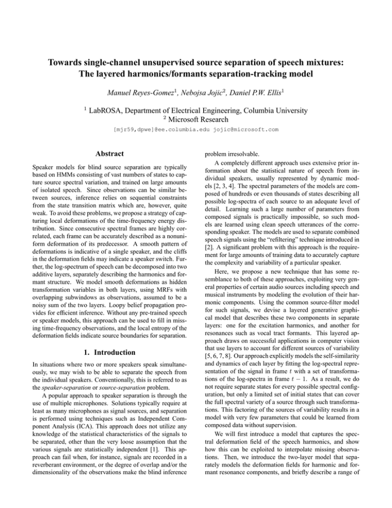
how this can be exploited to interpolate missing observations. Then, we introduce the two-layer model that separately models the deformation fields for harmonic and formant resonance components, and briefly describe a range of
1
9
X9t
Xt-1
8
Xt-1
X8t
Transformation
7
matrix T
Xt-1
X7t
6
Xt-1
Xt6
00100
5
= Xt5
0 0 0 1 0 • Xt-1
4
00001
Xt-1
Xt4
3
X3t
NP=5 Xt-1
2
Xt-1
X2t
1
Xt-1
X1t
Figure 3: Example transformation map showing corresponding points on original signal.
X15
X50
TT13
X14
X04
TT22
TT12
X13
X30
X12
X20
frequency
X
TT23
T13
t
T12
t-1
TT11
X11
X10
time
Figure 2: a) Graphical model b) Graphical simplification.
existing applications including semi-supervised source separation. Finally we describe the matching-tracking model including the initial states, and discuss its application to the
unsupervised source separation task.
2. Spectral Deformation Model
Figure 1 shows a narrow band spectrogram representation
of a speech signal, where each column depicts the energy
content across frequency in a short-time window, or timeframe. The value in each cell is actually the log-magnitude
of the short-time Fourier transform; in deciBels, Xtk =
PNF −1
−j2πτ k/NF
, where t is the timeτ =0 w[τ ]x[τ − t · H]e
frame index, k indexes the frequency bands, NF is the size of
the discrete Fourier transform, H is the hop between successive time-frames, w[τ ] is the NF -point short-time window,
and x[τ ] is the original time-domain signal. We use 32 ms
windows with 16 ms hops.
Using the subscript C to designate current and P to indicate previous, the model predicts a patch of NC timefrequency bins centered at the k th frequency bin of frame
t as a “transformation” of a patch of NP bins around the k th
bin of frame t − 1, i.e.
[k−nC ,k+nC ]
Xt
[k−nP ,k+nP ]
≈ Tkt · Xt−1
Blue:
Downward motion
(darker is steeper)
NC=3
T
T
T14
b) Transformation Map
a) Signal
b)
T15
Yellow/Orange:
Upward motion
(darker is steeper)
3
Figure 1: The NC = 3 patch of time-frequency bins outlined
in the spectrogram can be seen as an “upward” version of the
marked NP = 5 patch in the previous frame. This relationship can be described using the matrix shown.
a)
Green:
Identity transform
2
(1)
where nC = (NC − 1)/2, nP = (NP − 1)/2, and Ttk is
the particular NC × NP transformation matrix employed at
that point on the time-frequency plane. We use overlapping
patches to enforce transformation consistency [8].
Figure 1 uses an example with NC = 3 and NP = 5
to illustrate the intuition behind this approach. The selected
patch in frame t can be seen as a close replica of an upward
shift of part of the patch highlighted in frame t − 1. This
“upward” relationship can be captured by a transformation
matrix such as the one shown in the figure. The patch in
frame t − 1 is larger than the patch in frame t to permit both
upward and downward motions. The generative graphical
model for a single layer is depicted in figure 2. Nodes X =
{X11 , X12 , ..., Xtk , ..., XTK } represent all the time-frequency
bins in the spectrogram. For now, we consider the continuous
nodes X as observed, although below we will allow some of
them to be hidden when analyzing the missing data scenario.
Discrete nodes T = {T11 , T12 , ..., Ttk , ..., TTK } index the set
of transformation matrices used to model the dynamics of
the signal. Each NC × NP transformation matrix T is of the
form:
w 0 0
0 w 0
(2)
00 w
i.e. each of the NC cells at time t predicted by this matrix is
based on the same transformation of cells from t − 1, translated to retain the same relative relationship. Here, NC = 3
and w is a row vector with length NW = NP − 2; using
w = (0 0 1) yields the transformation matrix shown in figure 1. To ensure symmetry along the frequency axis, we constraint NC , NP and NW to be odd. The complete set of
w vectors include upward/downward shifts by whole bins as
well as fractional shifts. An example set, containing each w
vector as a row, is:
 0 0 0 0 1 


0
0
0
0
.
.75
1
0
0
0
0
.
.25
0
0
0
0
.25
.
0
0
.25
.75
1
.75
.
0
0
.75
.25
0 
0 
.
0
0
(3)
The length NW of the transformation vectors defines the sup[k−n ,k+nW ]
porting coefficients from the previous frame Xt−1 W
(where nW = (NW − 1)/2) that can “explain” Xtk .
For harmonic signals in particular, we have found that
a model using the above set of w vectors with parameters
NW = 5, NP = 9 and NC = 5 is very successful at capturing the self-similarity and dynamics of the harmonic structure. The transformations set could, of course, be learned,
but in view of the results we have obtained with this predefined set, we defer the learning of the set to future work.
b) Missing Data
a) Original
c) After iteration 10
d) After iteration 30
Figure 5: Missing data interpolation example a) Original, b) Incomplete, c) After 10 iterations, d) After 30.
Clean Formants Map
Clean Signal
Noisy Signal
Noisy Formants Map
Figure 6: Formant tracking map for clean speech (left panels) and speech in noise (right panels).
t-1
t
t
t-1
TH
TF
F
X
H
Figure 4: Graphical representation of the two-layer sourcefilter transformation model.
The clique “local-likelihood” potential between the timefrequency bin Xtk , its relevant neighbors in frame t, its relevant neighbors in frame t − 1, and its transformation node
Ttk has the following form:
[k−n ,k+nC ]
[k−n ,k+nP ]
ψ Xt C
, Xt−1 P
, Ttk =
[k−n ,k+nC ]
[k−n ,k+nP ]
N Xt C
; Tkt Xt−1 P
, Σ[k−nC ,k+nC ]
(4)
Diagonal matrix Σ[k−nC ,k+nC ] , which is learned, has different values for each frequency band to account for the variability of noise across frequency bands. For the transformation cliques, the horizontal and vertical transition potenk
tials ψhor (Ttk , Tt−1
) and ψver (Ttk , Ttk−1 ), are represented
by transition matrices.
For observed nodes X , inference consists in finding
probabilities for each transformation index at each timefrequency bin. Exact inference is intractable and is approximated using Loopy Belief Propagation [9, 10]. Appendix
A gives a quick review of the loopy belief message passing
rules, and Appendix B presents the specific update rules for
this case. The transformation map, a graphical representation
of the modes of the transformation node posteriors across
time-frequency, provides an appealing description of the harmonics’ dynamics as can be observed in figure 3. In these
panels, the links between three specific time-frequency bins
and their corresponding transformations on the map are highlighted. Bin 1 is described by a steep downward transformation, while bin 3 also has a downward motion but is described
by a less steep transformation, consistent with the dynamics
visible in the spectrogram. Bin 2, in other hand, is described
by a steep upwards transformation. These maps tend to be
robust to noise (as shown below), making them a valuable
representation in their own right.
3. Inferring Missing Data
If a certain region of cells in the spectrogram are missing, the
corresponding nodes in the model become hidden. This is illustrated in figure 5, where a rectangular region in the center
has been removed and tagged as missing. Loopy belief inference now requires continuous-valued messages, complicating the procedure as explained in Appendix C. The figure
shows the interpolated values inferred by the model after a
few iterations. The missing-data model will be used below
in the two layer source-filter model.
4. Two Layer Source-Filter Transformations
Many sound sources, including voiced speech, can be successfully regarded as the convolution of a broad-band source
excitation, such as the pseudo-periodic glottal flow, perhaps
modeled as an impulse train, and a time-varying resonant
filter, such as the vocal tract, that ‘colors’ the excitation to
produce speech sounds or other distinctions. When the excitation has a spectrum consisting of well-defined harmonics, the overall spectrum is in essence samples of the filter’s
resonances at the frequencies of the harmonics. Convolution of the source with the filter in the time domain corresponds to multiplying their spectra in the Fourier domain, or
an additive relationship in the log-spectral domain. Hence,
=
+
Harmonics
Signal
Selected Bin
Harmonic Tracking
a).
b).
Formants
Formant Tracking
c).
Figure 7: First row: Harmonics/Formants decomposition (posterior distribution means). Row 2: Harmonics/Formants tracking
example. The transformation maps on both layers are used to track a given time-frequency bin. Row 3: Semi-supervised Two
Speakers Separation. a) The user selects bins on the spectrogram that she believes correspond to one speaker. b) The system finds
the corresponding bin on the transformation map. c) The system selects all bins whose transformations match the ones chosen;
the remaining bins correspond to the other speaker.
we model the log-spectra X as the sum of variables F and
H, which explicitly model the formants and the harmonics
of the speech signal. The source-filter transformation model
is based on two additive layers of the deformation model described above, as illustrated in figure 4. Variables F and H in
the model are hidden, while, as before, X can be observed or
hidden. The symmetry between the two layers is broken by
using different parameters in each, chosen to suit the particular dynamics of each component. We use transformations
with a larger support in the formant layer (NW = 9) compared to the harmonics layer (NW = 5). Since all harmonics tend to move in the same direction, we enforce smoother
transformation maps on the harmonics layer by using potential transition matrices with a higher self-loop probabilities.
An example of the transformation map for the formant layer
is shown in figure 6, which illustrates how these maps can remain relatively invariant to high levels of signal corruption;
belief propagation searches for some kind of consistent dynamic structure within the signal, and since additive noise is
less likely to have a well-organized structure, it is properties
of the speech component that are extracted. Inference in this
model is more complex, but the actual form of the continuous messages is essentially the same as in the one layer case
(Appendix C), with the addition of the potential function relating the signal Xtk with its transformation components Htk
and Ftk ) at each time-frequency bin:
ψ(Xtk , Htk , Ftk ) = N (Xtk ; Htk + Ftk , σ k )
(5)
The first row of figure 7 shows the decomposition of a speech
signal into harmonics and formants components, illustrated
as the means of the posteriors of the continuous hidden variables in each layer.
5. Applications
We have built an interactive model that implements formant and harmonics tracking, missing data interpolation, formant/harmonics decomposition, and semi-supervised source
separation of two speakers.
Formants and Harmonics Tracking: Analyzing a signal with the two-layer model permits separate tracking of the
harmonic and formant ‘ancestors’ of any given point. The
user clicks on the spectrogram to select a bin, and the system
reveals the harmonics and formant “history” of that bin, as
illustrated in the second row of figure 7.
Semi-Supervised Source Separation: After modeling
the input signal, the user clicks on time-frequency bins that
appear to belong to a certain speaker. The demo then masks
all neighboring bins with the same value in the transformation map; the remaining unmasked bins should belong to the
other speaker. The third row of figure 7 depicts an example with the resultant mask and the “clicks” that generated it.
Although far from perfect, the separation is good enough to
perceive each speaker in relative isolation.
Missing Data Interpolation and Harmonics/Formants
Separation: Examples of these have been shown in figures
5 and 7.
St
St+1 St+2
F
H
TF
k-1
T t-1
TH
k-1
l t-1
f
x
k-1
t-1
g
t
l tk-1
k-1
v t-1
k-1
t-1
k
T t-1
t+1
l
Xt+1
a) Matching-Tracking Model
Composed Signal
x
v tk-1
k-1
t
k-1
t-1
t
t+1
T tk-1
k-1
h t-1
x
k
h t-1
T tk
l tk
k
t-1
k
t-1
x
k
t
b) Factor Graph
Entropy Maps
Entropy Edges
Figure 8: First row: Graphic model and factor graph of the matching-tracking model; Second row: Entropy Map and Entropy
Edges
Features for Speech Recognition: The phonetic distinctions at the basis of speech recognition reflect vocal tract filtering of glottal excitation. In particular, the dynamics of
formants (vocal tract resonances) are known to be powerful
“information-bearing elements” in speech. We believe the
formant transformation maps may be a robust discriminative
feature to be use in conjunction with traditional features in
speech recognition systems, particularly in noisy conditions;
this is future work.
lows: When multiple speakers are present, each speaker will
be modeled in its own layer, further divided into harmonics
and formants layers. The idea is to reduce the transformation uncertainty at the onset of occlusions by continuing the
tracking of the “old” speaker in one layer at the same time
as estimating the initial state of the “new” speaker in another
layer – a realization of the “old-plus-new” heuristic from psychoacoustics. This is part of our current research.
7. Conclusions
6. Matching-Tracking Model
The second row of figure 8 b) illustrates the entropy of the
distributions inferred by the system for each transformation
variable. The third pane shows ‘entropy edges’, boundaries
of high transformation uncertainty. With some exceptions,
these boundaries correspond to transitions between silence
and speech, or when occlusion between speakers starts or
ends. Similar edges are also found at the transitions between
voiced and unvoiced speech. High entropy at these points
indicates that the model does not know what to track, and
cannot find a good transformation to predict the following
frames. This motivates the introduction of a new variable in
the model to provide a set of explicit “initial states”. We refer
to this as the “matching-tracking” model, represented graphically in the first row of figure 8. One state/switch variable
St per time frame is connected as a regular HMM on top of
the two tracking layers. But unlike a regular HMM, the S
variables have a special “tracking state” in which the model
tracks the current observation values through deformations
instead of matching it to the most likely template. Hence, the
model requires only a small set of states, with a few states
representing the pitch of the speaker and a few others for unvoiced sounds.
The source separation problem can be addressed as fol-
We have presented a harmonic/formant separation and tracking model that effectively identifies the different factors underlying speech signals. We show that this model has a number of useful applications, many of which have already been
implemented in a working real-time demo. Previous research
has shown that single-microphone speech source separation
is possible given detailed models of the sources, but learning
those models in a unsupervised way from composed signals
is practically impossible. The model we have proposed in
this paper captures the detailed dynamics of speech with only
a few parameters, and is a promising candidate for sound separation systems that do not rely on extensive isolated-source
training data.
8. Appendices
A: Loopy Belief Propagation
The sum-product algorithm [12] can be used to approximate
inference on graphical models with loops. The algorithm update rules applied to the factor graph representation of the
model are:
Variable to local function:
Y
mx→f (x) =
mf →x (x)
(6)
h∈n(x)\f
Local function to variable:
X
mf →x (x) =
f (X)
∼x
Y
my→f (y)
(7)
y∈n(f )\x
where X = n(f ) is the set of arguments of the function f .
The factor graph for a section of our model is depicted
in the top right corner of figure 8. The circles are the variable nodes, representing the hidden variables, and the squares
represent the local function nodes, i.e. the potential functions within variable nodes [12]. The solid lines represent
the model when the variables Xtk are observed, and the dotted part is added when they are hidden.
B: Update Rules for the Spectral Deformation Model
When variables Xtk are observed, there are only discrete
messages in the algorithm. Applying the above update rules,
we obtain the following forward recursion for the horizontal
nodes on the grid:
X
k
k
(Tt−1
))
mTtk →hkt (Ttk ) = (
hkt (Ttk , Tt−1
)mTt−1
k →hk
t−1
k
Tt−1
The values displayed by the missing data application are
these mean values. The variable to local functions have the
same form as in equation 10, just subtracting the numerator
and denominator factor corresponding to the incoming message from the corresponding function. Since we use diagonal
variances, parameters µy and µz in 9 are found by concatenating the relevant µX parameters. When using the two layer
model, an extra message comes from node gtk adding extra
factors in the numerator and denominator of equation 10.
9. Acknowledgments
This work was supported by Microsoft Research and by the
NSF under grant no. IIS-0238301. Any opinions, findings
and conclusions or recommendations expressed in this material are those of the author(s) and do not necessarily reflect
the views of the NSF.
10. References
[1]
A. Hyvärinen, ”Survey on Independent Component
Analysis”, Neural Computing Surveys, 1999.
[2]
S. Roweis, ”One-microphone source separation”, Advances in NIPS, MIT Press, 2000.
[3]
S. Roweis, ”Factorial Models and refiltering for Speech
Separation and Denoising”, Proc. EuroSpeech, Geneva,
2003.
[4]
M. Reyes-Gomez, D. Ellis, and N. Jojic, ”Subband audio modeling for single-channel acoustic source separation”, Proc. ICASSP, Montreal, 2004.
[5]
N. Jojic and B. Frey, ”Learning flexible sprites in video
layers”, Proc. CVPR, 2001.
[6]
A. Lenit, A. Zomet, and Y. Weiss ”Learning to perceive transparency from the statistics of natural scenes”,
Proc. NIPS, 2002.
[7]
P.H.S. Torr, R. Szeliski, and P. Anandan, ”An integrated
Bayesian approach in layer extraction from sequences”,
PAMI, 2001.
[8]
N. Jojic, B. Frey, and A. Kannan, ”Epitomic Analysis
of Appearance and Shape”, Proc. ICCV, 2003.
[9]
J.S. Yedidia, W.T. Freeman, and Y. Weiss, ”Understanding Belief Propagation and its Generalizations”,
Exploring Artificial Intelligence in the New Millennium, Chapter 8.
[k−NC :k+NC ]
[k−n :k+nP ]
ltk (Xt
, Xt−1 P
, Ttk )g(Ttk−1 , Ttk+1 )
(8)
where g(Ttk−1 , Ttk+1 ) is the multiplication of the messages
coming from the adjacent vertical nodes. A similar backward
recursion can also be found. The messages for the vertical
chains can be updated through analogous upward/downward
recursions.
C: Loopy Belief with Continuous-Valued Messages
The message from function lsr of the factor graph in figure 8
to variable Xji has the form.
mlsr →Xji (Xji ) =
Z
0
1
1
(αXji −Γy+z) Σ−1
(αXij −Γy+z)
[r−nC :r+nC ]
exp 2
C
y,z
N (y; µy , Σy )N (z; µz , Σz )dydz
(9)
Values j and s can be either t or t − 1, and vector y is
[r−n :r+nP ]
formed by the values on Xt−1 P
other than Xji (or
[r−N :r+N ]
C
C
the whole vector if j = t). Vectors z and Xt
have an analogous relationship. Vector α and matrix Γ come
from the most likely (or weighted mean) of the transformation matrix used at bin Xsr . To speed up the process, we
approximate N (y; µy , Σy )N (z; µz , Σz ) by delta functions
δ(y − µy ) and δ(z − µz ). Then the messages reduce to:
0
i
−1
1
(αXji −Γµy +µz )
1
2 (αXj −Γµy +µz ) Σ
.
C exp
k
k
posterior probability of node Xt , q(Xt ), is equal
mlsr →Xji (Xji ) =
The
to the multiplication of all its incoming messages. We approximate this multiplication with a Gaussian distribution,
0
q (Xtk ) = N (Xtk ; µXtk , ψXtk ). Minimizing their KL divergence we find:
PNC +NP 0 −1
αi Σi (Γi yi − zi )
µXtk = i=1
(10)
PNC +NP 0 −1 −1
αi Σi αi
i=1
[10] Y. Weiss and W.T. Freeman, ”Correctness of Belief
Propagation in Gaussian Graphical Models of Arbitrary
Topology”, Neural Computation, V13, No 10, pp 21732200, 2001.
[12] F. Kschischang, B. Frey, and H.-A. Loeliger, ”Factor
Graphs and the Sum-Product Algorithm”, IEEE Transactions on information theory, Vol. 47 No. 2, 2001.