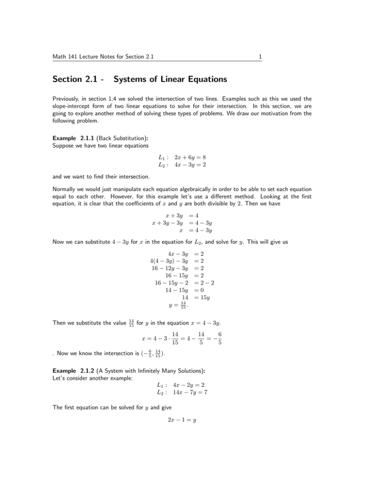
Math 141 Lecture Notes for Section 2.1
Section 2.1 -
1
Systems of Linear Equations
Previously, in section 1.4 we solved the intersection of two lines. Examples such as this we used the
slope-intercept form of two linear equations to solve for their intersection. In this section, we are
going to explore another method of solving these types of problems. We draw our motivation from the
following problem.
Example 2.1.1 (Back Substitution):
Suppose we have two linear equations
L1 :
L2 :
2x + 6y = 8
4x − 3y = 2
and we want to find their intersection.
Normally we would just manipulate each equation algebraically in order to be able to set each equation
equal to each other. However, for this example let’s use a different method. Looking at the first
equation, it is clear that the coefficients of x and y are both divisible by 2. Then we have
x + 3y = 4
x + 3y − 3y = 4 − 3y
x = 4 − 3y
Now we can substitute 4 − 3y for x in the equation for L2 , and solve for y. This will give us
4x − 3y
4(4 − 3y) − 3y
16 − 12y − 3y
16 − 15y
16 − 15y − 2
14 − 15y
14
14
y = 15
.
Then we substitute the value
14
15
=2
=2
=2
=2
=2−2
=0
= 15y
for y in the equation x = 4 − 3y.
x=4−3·
14
14
6
=4−
=−
15
5
5
. Now we know the intersection is (− 65 , 14
15 ).
Example 2.1.2 (A System with Infinitely Many Solutions):
Let’s consider another example:
L1 : 4x − 2y = 2
L2 : 14x − 7y = 7
The first equation can be solved for y and give
2x − 1 = y
Math 141 Lecture Notes for Section 2.1
2
However, when we substitute into the second equation, we have:
14x − 7(2x − 1) = 7
14x − 14x + 7 = 7
7 =7
This last line is clearly true, however, this doesn’t help us solve for x. The reason this occurs is
because the two lines have infinitely many solutions. In order to still give a usable answer to list the
set of solutions for these two linear equations we use a method called parameterization. We choose
a variable (commonly t) called the parameter and create equations for the two variables in our lines
that are in the form of t. In this example, we have the equations:
x=t
y = 2t − 1
and
This lets us say that all solutions of this system of linear equations are points of the form (t, 2t − 1)
where t is any real number.
Example 2.1.3 (A System with No Solutions):
As a third example, consider the system of linear equations:
L1 :
L2 :
2x +4y
3x +6y
First, from L1 we can obtain
x=
=9
= 12
9
− 2y
2
and by substitution we have
9
27
27
12 = 3( − 2y) + 6y =
− 6y + 6y =
.
2
2
2
Unfortunately this equation is always false. Since the equality 12 = 27
2 is never true, there must be
no solutions so we know that L1 and L2 have no intersection, and we write DN E to show that no
solution exists.
An equation of the form
Ax + By + Cz = D
where A, B, C, and D are all constants and not all of A, B, and C are zero is the equation of a plane.
We can also solve systems of equations in three variables using the methods explored in the three
examples above. In fact, we aren’t limited to three variables, we can use as many variables as we like.
We are still limited by the possibilities of one, zero, or infinitely many solutions.
Example 2.1.4 (A System with More than Two Variables):
Consider the following equations
P1 :
P2 :
P3 :
2x
x
3x
+3y
+2y
+4y
+5z
−4z
−z
=6
=1
= −4
Math 141 Lecture Notes for Section 2.1
3
Now, we need to solve for a variable and substitute. Here the first variable that can be clearly isolated
is x from P2 which can be solved to find
x = 1 − 2y + 4z
Substituting into P1 gives us
2(1 − 2y + 4z) + 3y + 5z
2 − 4y + 8z + 3y + 5z
2 − y + 13z
13z − 4
=6
=6
=6
=y
We can then use both substitutions into P3 to obtain:
3(1 − 2y + 4z) + 4y − z
3 − 6y + 12z + 4y − z
3 − 2y + 11z
3 − 2(13z − 4) + 11z
3 − 26z + 8 + 11z
11 − 15z
−15z
z
= −4
= −4
= −4
= −4
= −4
= −4
= −15
= 1.
Then we can solve for y with y = 13(1) − 4 = 9, and lastly x = 1 − 2(9) + 4(1) = 5 − 18 = −13. Thus
our solution is the point (−13, 9, 1) and we are done.
Suggested Homework Problems: 5, 7, 9, 11, 19, 23, 27, 31, 35, 37, 39.