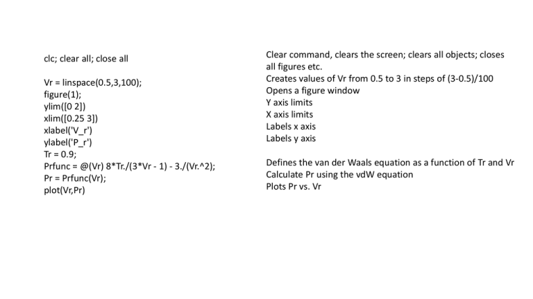
clc; clear all; close all
Vr = linspace(0.5,3,100);
figure(1);
ylim([0 2])
xlim([0.25 3])
xlabel('V_r')
ylabel('P_r')
Tr = 0.9;
Prfunc = @(Vr) 8*Tr./(3*Vr - 1) - 3./(Vr.^2);
Pr = Prfunc(Vr);
plot(Vr,Pr)
Clear command, clears the screen; clears all objects; closes
all figures etc.
Creates values of Vr from 0.5 to 3 in steps of (3-0.5)/100
Opens a figure window
Y axis limits
X axis limits
Labels x axis
Labels y axis
Defines the van der Waals equation as a function of Tr and Vr
Calculate Pr using the vdW equation
Plots Pr vs. Vr
if Tr < 1
Makes sure the temperature is below critical, Tr = T/Tc
Pr_b = 1.0;
Starts with a trial value for Pr at which liquid transform to gas
vdW_Pr_b = [1 -1/3*(1+8*Tr/Pr_b) 3/Pr_b -1/Pr_b];
Defines a polynomial function to calculate the values of Vr for the
trial value of Pr (Pr_b).
8𝑇𝑟
3
⇒
−
= 𝑃𝑟𝑏
3𝑉𝑟 − 1 𝑉𝑟2
⇒
8𝑇𝑟
3
− 2 − 𝑃𝑟𝑏 = 0
3𝑉𝑟 − 1 𝑉𝑟
⇒ 8𝑇𝑟 𝑉𝑟2 − 3 3𝑉𝑟 − 1 − 𝑃𝑟𝑏 3𝑉𝑟 − 1 𝑉𝑟2 = 0
⇒ 8𝑇𝑟 𝑉𝑟2 − 9𝑉𝑟 + 3 − 3𝑃𝑟𝑏 𝑉𝑟3 + 𝑃𝑟𝑏 𝑉𝑟2 = 0
1
8𝑇𝑟 2
3
1
1+
𝑉𝑟 +
𝑉𝑟 −
=0
3
𝑃𝑟𝑏
𝑃𝑟𝑏
𝑃𝑟𝑏
The terms in the square brackets are the coefficients of the
polynomial.
⇒ 𝑉𝑟3 −
v = sort(roots(vdW_Pr_b));
Finds the roots of the polynomial and sorts them in
increasing order: v(1), v(2), and v(3)
A1 = (v(2)-v(1))*Pr_b - integral(Prfunc,v(1),v(2));
A2 = integral(Prfunc,v(2),v(3)) - (v(3)-v(2))*Pr_b;
2.5
2
1.5
1
0.5
0
0.5
1
1.5
2
2.5
3
Calculates the area enclosed by the line and the vdW
curve between v(1) and v(2) and then from v(2) and v(3).
(clearer figure later).
Z = abs(A1-A2);
while Z > 0.0001
vdW_Pr_b = [1 -1/3*(1+8*Tr/Pr_b) 3/Pr_b -1/Pr_b];
v = sort(roots(vdW_Pr_b));
Prfunc = @(Vr) 8*Tr./(3*Vr - 1) - 3./(Vr.^2);
A1 = (v(2)-v(1))*Pr_b - integral(Prfunc,v(1),v(2));
A2 = integral(Prfunc,v(2),v(3)) - (v(3)-v(2))*Pr_b;
Z = abs(A1 - A2);
Pr_b = Pr_b - 0.00001;
figure(1); hold off;
plot(Vr,Pr)
figure(1); hold on;
plot([0.5 3],[Pr_b Pr_b],'k--')
hold off;
end
Calculates the difference between the two areas
If z > 0.0001 then this loop starts
Defines the polynomial in the loop
Calculates and sorts the roots
Defines vdW equation in the loop
Calculates the areas again
Calculates the difference
Lowers the test values Pr_b by 0.00001
Chooses figure 1 window; new plot will appear, old graph is removed
Plots Pr vs. Vr
Chooses figure 1window; new plot will appear keeping the old graph
Plots the line for Pr_b vs. Vr in a black dashed line
Next time a new graph is plotted the old plots will be removed
Starts the loop again and checks if the difference between A1 and A2
(Z) > 0.0001 for the new value of Pr_b. Loop stops if Z < 0.0001 i.e
A1  A2
2.5
2
1.5
1
v(1)
v(3)
v(2)
Pr_b
0.5
0
0.5
1
(v(2)-v(1))*Pr_b
1.5
2
(v(3)-v(2))*Pr_b
2.5
3
2.5
2
1.5
1
v(1)
v(3)
v(2)
Pr_b
0.5
0
0.5
1
integral(Prfunc,v(1),v(2))
1.5
2
integral(Prfunc,v(2),v(3))
2.5
3
Calculates the area under the vdW curve from
v(1) to v(2) and from v(2) to v(3).
2.5
2
1.5
1
v(1)
v(3)
v(2)
Pr_b
0.5
0
0.5
1
1.5
2
(v(2)-v(1))*Pr_b - integral(Prfunc,v(1),v(2))
integral(Prfunc,v(2),v(3)) - (v(3)-v(2))*Pr_b
2.5
3
Calculates the relevant area for the Maxwell
constructions
end
A1
A2
Pr_b
Ends the if loop
Prints A1 and A2
Prints the value of pressure Pr_b which satisfies Maxwell’s condition.