Solutions to BU7527 exam (December 2013)
mjp@maths.tcd.ie
December 18, 2013
1. (a)
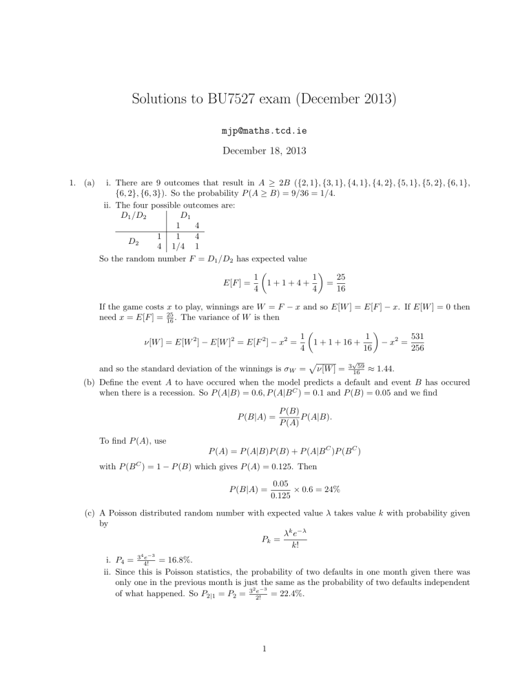
i. There are 9 outcomes that result in A ≥ 2B ({2, 1}, {3, 1}, {4, 1}, {4, 2}, {5, 1}, {5, 2}, {6, 1},
{6, 2}, {6, 3}). So the probability P (A ≥ B) = 9/36 = 1/4.
ii. The four possible outcomes are:
D1 /D2
D1
1
4
1
1
4
D2
4 1/4 1
So the random number F = D1 /D2 has expected value
1
25
1
1+1+4+
=
E[F ] =
4
4
16
If the game costs x to play, winnings are W = F − x and so E[W ] = E[F ] − x. If E[W ] = 0 then
need x = E[F ] = 25
16 . The variance of W is then
1
1
531
ν[W ] = E[W 2 ] − E[W ]2 = E[F 2 ] − x2 =
1 + 1 + 16 +
− x2 =
4
16
256
and so the standard deviation of the winnings is σW =
p
ν[W ] =
√
3 59
16
≈ 1.44.
(b) Define the event A to have occured when the model predicts a default and event B has occured
when there is a recession. So P (A|B) = 0.6, P (A|B C ) = 0.1 and P (B) = 0.05 and we find
P (B|A) =
P (B)
P (A|B).
P (A)
To find P (A), use
P (A) = P (A|B)P (B) + P (A|B C )P (B C )
with P (B C ) = 1 − P (B) which gives P (A) = 0.125. Then
P (B|A) =
0.05
× 0.6 = 24%
0.125
(c) A Poisson distributed random number with expected value λ takes value k with probability given
by
λk e−λ
Pk =
k!
4 −3
e
i. P4 = 3 4!
= 16.8%.
ii. Since this is Poisson statistics, the probability of two defaults in one month given there was
only one in the previous month is just the same as the probability of two defaults independent
2 −3
e
of what happened. So P2|1 = P2 = 3 2!
= 22.4%.
1
iii. Pk≥4 = P0 + P1 + P2 + P3 + P4
0
1
2
3
4
Sum
115e
60 e−6
0!
61 e−6
1!
62 e−6
2!
63 e−6
3!
64 e−6
4!
−6
= 28.5%
2. (a)
1
Z
dr
fQ (q) =
0
r=1
r2
1
q + r = qr +
=q+
2 r=0
2
(b)
1
Z
E[Q] =
dq
3
q=1
7
q
q
q2
q + =
=
+
2
3
2 q=0
12
1
Z
qfQ (q) =
2
dq
0
0
Since ν[Q] = E[Q2 ] − E[Q]2 and
2
Z
1
E[Q ] =
dq
4
q=1
q
q3
5
q2
=
+
=
q +
2
4
6 q=0
12
1
Z
2
q fQ (q) =
3
dq
0
0
then
ν[Q] =
5
−
12
7
12
2
=
11
144
(c) Using P (Q < 1/2|R > 1/2) = P (Q < 1/2 ∩ R > 1/2)/P (R > 1/2) with
Z
1
P (R > 1/2) =
1
Z
P (Q < 1/2 ∩ R > 1/2) =
dr
1/2
1
0
dq
q+r =
0
1
q2
+ qr
q+r =
dr
2
1/2
Z
dq
1
dr
1/2
Z
Z
5
,
8
q=1/2
q=0
r2
r
=
+
4
8
r=1
=
r=1/2
gives
2
5
and then P (Q < 1/2|R ≤ 1/2) = P (Q < 1/2 ∩ R ≤ 1/2)/P (R ≤ 1/2) with
P(Q < 1/2|R > 1/2) =
P (R ≤ 1/2) = 1 − P (R > 1/2) =
P (Q < 1/2 ∩ R ≤ 1/2) =
1
8
P(Q < 1/2|R ≤ 1/2) =
1
3
3
8
gives
3. See spreadsheet
4. (a)
i. Since
1
1
1
E[Xk+1 ] = p(E[Xk ] + 3) + (E[Xk ] + 1) + ( − p)(E[Xk ] − 2) = E[Xk ] + 5p −
2
2
2
and for Xk to be a martingale means E[Xk+1 ] = E[Xk ] requires 5p =
2
1
2
or p =
1
10 .
1
4
ii. For a martingale, E[XT ] = E[X0 ] when T is a stopping time. So E[XT ] = 4.
iii. Define q = P (XT = 20) = 1−P (XT = 0) then 20q+0×(1−q) = 4 implies P(XT = 20) = 15 and
P(XT = 0) = 45 . The variance of XT is then ν[XT ] = E[XT2 ]−E[XT ]4 = ( 15 ×202 + 45 ×02 )−42 =
64.
iv. The system is described by a Markov matrix:

 1
0 14
2
M =  21 23 0 
0 13 34
and the fixed point obeys M π = π with π1 + π2 + π3 =. First find M w = w with w1 = 1 and
rescale later. This gives 21 + 14 w3 = 1 and 12 + 23 w2 = w2 which implies w2 = 23 and w3 = 2.
Rescaling to put back the probability constraint gives
 2 

π=
3
9
1
3
4
9

