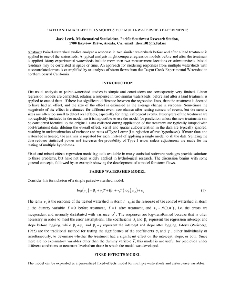
FIXED AND MIXED-EFFECTS MODELS FOR MULTI-WATERSHED EXPERIMENTS
Jack Lewis, Mathematical Statistician, Pacific Southwest Research Station,
1700 Bayview Drive, Arcata, CA, email: jlewis01@fs.fed.us
Abstract: Paired-watershed studies analyze a response in two similar watersheds before and after a land treatment is
applied to one of the watersheds. A typical analysis might compare regression models before and after the treatment
is applied. Many experimental watersheds include more than two measurement locations or subwatersheds. Model
residuals may be correlated in space or time. An approach for modeling responses from multiple watersheds with
autocorrelated errors is exemplified by an analysis of storm flows from the Caspar Creek Experimental Watershed in
northern coastal California.
INTRODUCTION
The usual analysis of paired-watershed studies is simple and conclusions are consequently very limited. Linear
regression models are computed, relating a response in two similar watersheds, before and after a land treatment is
applied to one of them. If there is a significant difference between the regression lines, then the treatment is deemed
to have had an effect, and the size of the effect is estimated as the average change in response. Sometimes the
magnitude of the effect is estimated for different event size classes after testing subsets of events, but the sample
sizes are often too small to detect real effects, especially for large, infrequent events. Descriptors of the treatment are
not explicitly included in the model, so it is impossible to use the model for prediction unless the new treatments can
be considered identical to the original. Data collected during application of the treatment are typically lumped with
post-treatment data, diluting the overall effect. Serial and spatial autocorrelation in the data are typically ignored,
resulting in underestimation of variance and rates of Type I error (i.e. rejection of true hypotheses). If more than one
watershed is treated, the analysis is repeated for each, instead of applying a single model to all the data. Splitting the
data reduces statistical power and increases the probability of Type I errors unless adjustments are made for the
testing of multiple hypotheses.
Fixed and mixed-effects regression modeling tools available in many statistical software packages provide solutions
to these problems, but have not been widely applied in hydrological research. The discussion begins with some
general concepts, followed by an example showing the development of a model for storm flows.
PAIRED WATERSHED MODEL
Consider this formulation of a simple paired-watershed model:
log ( y j ) = β0 + γ 0T + (β1 + γ1T ) log ( yCj ) + ε j
(1)
The term y j is the response of the treated watershed in storm j, yCj is the response of the control watershed in storm
j, the dummy variable T = 0 before treatment, T = 1 after treatment, and ε j ∼ N (0, σ2 ) , i.e. the errors are
independent and normally distributed with variance σ2 . The responses are log-transformed because that is often
necessary in order to meet the error assumptions. The coefficients β0 and β1 represent the regression intercept and
slope before logging, while β0 + γ 0 and β1 + γ1 represent the intercept and slope after logging. F-tests (Weisberg,
1985) are the traditional method for testing the significance of the coefficients γ 0 and γ1 , either individually or
simultaneously, to determine whether the treatment had a significant effect on the intercept, slope, or both. Since
there are no explanatory variables other than the dummy variable T, this model is not useful for prediction under
different conditions or treatment levels than those in which the model was developed.
FIXED-EFFECTS MODEL
The model can be expanded as a generalized fixed-effects model for multiple watersheds and disturbance variables:
log ( yij ) = β0i + f 0 ( x, γ 0 ) + (β1i + f1 ( x, γ1 ) ) log ( yCj ) + εij
(2)
The subscript i indexes treated watersheds. The term yCj could represent an average response from one or more
control watersheds. (Individual terms for each control watershed are probably not generally warranted, because of
the complexity and loss of degrees of freedom.) β0i and β1i can be termed “location parameters” since there is one
for each treated watershed. The disturbance functions f0 and f1 replace the dummy treatment variables of the paired
watershed model. They are functions of variables describing watershed condition (vector x ) and “disturbance
parameters” (vectors γ 0 and γ1 ). The error assumptions, too, can be relaxed using the multivariate normal
distribution to model correlated errors and heterogeneous variance, as εij ∼ N(0, Σ) , where Σ is an n × n
covariance matrix (n is the total number of observations yij ).
MIXED-EFFECTS MODEL
If some of the fixed effects are replaced with random effects, the result is a mixed-effects model:
log ( yij ) = β0 + b0i + f 0 ( x, γ 0 ) + (β1 + b1i + f1 ( x, γ1 ) ) log ( yCj ) + εij
(3)
Here, the location parameters β0i and β1i are replaced by a mean slope β0 , mean intercept, β1 , and random
effects, b0i and b1i , representing deviations from β0 and β1 , respectively. The random effects are assumed to follow
a bivariate normal distribution, i.e. b ∼ N(0, Σb ) . For independent random effects the 2 × 2 covariance matrix Σb is
a diagonal matrix containing just the variances of b0i and b1i . For correlated random effects the matrix also includes
a non-zero covariance. (Typically slopes and intercepts are negatively correlated, so a watershed with a small slope
is likely to have a large intercept). The residual errors, εij ∼ N(0, Σ) , are assumed to be independent of the random
effects and independent between watersheds (hence Σ is block-diagonal, with watersheds as blocks). The random
effects and residual errors replace the more general error term of the fixed-effects model. The result is a model in
which errors within a watershed are correlated, but those between watersheds are independent.
If nw is the number of treated watersheds, then the 2nw location parameters of the fixed-effects model are replaced by
4 or 5 parameters in the mixed-effects model: β0 , β1 , and the 2 or 3 parameters in Σb . Therefore, if nw > 2 , the
mixed-effects model is more parsimonious than the fixed-effects model.
Using random effects is appropriate when one considers the subjects being parameterized (in this case watersheds)
to be a sample from some larger population, and it is the population rather than the particular sample that is the
focus of inference. Predictions for observations from unsampled watersheds require setting b0i = b1i = εij = 0 .
Estimates of potential variability (e.g. prediction intervals) consider both the variance of the random effects, Σb , and
the residual variance σ 2 .
EXAMPLE: MODELING STORM FLOW VOLUMES
To illustrate fitting of a mixed-effects model to multiple-watershed data, we use storm flow volumes (per unit area)
from the North Fork of Caspar Creek (Lewis et al., 2001) in California’s Jackson State Forest. In the North Fork
experiment, there were 13 gaged watersheds. Three were held as controls, five were clearcut, and five below the
clearcut stations included mixtures of cut and uncut areas. Pretreatment measurements were taken for four years,
logging took place over a three-year period, and measurements were continued for three more years at seven stations
and nine more years at six stations. The mean flow volume of two control watersheds was selected for use as a
synthetic control, because the two stations had been monitored for the entire duration of the study, and their mean
generally correlated with the treated watersheds (before treatment) better than either of their individual responses.
Models For The Mean Response: We start with a simple fixed-effects model that includes only slopes and
intercepts relating responses in the treated watersheds to the synthetic control. This model essentially fits a separate
linear regression for each watershed.
log ( yij ) = β0i + β1i log′ ( yCj ) + εij
(4)
m
where log′ ( yCj ) = log ( yCj ) − ∑ log ( yCj ) m is log ( yCj ) centered at its mean. Centering is necessary to make
j =1
meaningful comparisons of both intercepts and slopes. Otherwise the extrapolation of intercepts back to zero
induces large negative correlations between the intercepts and slopes. A display of 95% confidence intervals for
slopes and intercepts (figure 1) indicates that the intercepts are clearly different from one another, while the slopes
do not differ greatly. That suggests a model with one fixed effect each for slope and intercept, plus a random effect
for intercepts:
log ( yij ) = β0 + b0i + β1log ( yCj ) + εij
(5)
The random effect is assumed to be normally distributed, i.e. b0i ∼ N ( 0, σb2 0 ) . This model assumes a common slope
but allows random deviations in intercept for each watershed. In place of 20 parameters ( β0i and β1i ) in model (4),
we only need estimate 3 parameters ( β0 , β1 , and σb20 ) for model (5).
Figure 1 Estimated 95% confidence intervals for intercepts and slopes of model (4)
Previous studies have shown that changes in runoff after logging were greatest in fall and early winter when soil
moisture differences were greatest between logged and unlogged sites (Harr et al., 1975; Ziemer 1981). When
antecedent wetness is lowest in uncut areas, soil moisture differences are expected to be greatest. For this analysis,
we defined antecedent wetness on day k as wk = 0.97716wk −1 + rk , where rk is the daily mean flow at the South Fork
of Caspar Creek, a neighboring watershed with perennial streamflow. The decay coefficient corresponds to a 30-day
half-life in the absence of runoff. Examining the relation of residuals from model (5) with proportion harvested at
different levels of wetness, it is apparent that the effect of cutting is greatest under conditions of low antecedent
wetness (figure 2). This suggests an interaction as the product of harvest proportion and antecedent wetness. The
following model introduces fixed effects for the harvest/wetness interaction as well as harvest proportion by itself
and a harvest/storm size interaction.
log ( yij ) = β0 + b0i + β1log ( yCj ) +  γ1 + γ 2 w j + γ 3 log ( yCj ) cij + εij
(6)
The harvested proportion of watershed i at storm j is denoted by cij , and the regional antecedent wetness at storm j
is wj. Storm size is represented by log ( yCj ) , the log-transformed response in the control watershed. The
harvest/storm size interaction allows the slope of the simple regression between treated and control watersheds to
change with proportion harvested. Relating model (6) to the general mixed-effects model (3), we have x = ( c, w ) ,
f 0 ( x, γ 0 ) = γ1cij + γ 2 w j cij , and f1 ( x, γ1 ) = γ 3cij .
Figure 2 Interaction between proportion harvested and antecedent wetness in residuals from model (5)
Figure 3 Declining trend in residuals from model (6) resulting from regrowth after logging
Without a term to account for regrowth there is a declining trend in the residuals (figure 3). We can account for
regrowth by replacing the proportion harvested, cij , in model (6) with a term, xij , that diminishes linearly with time
after harvest:
log ( yij ) = β0 + b0i + β1log ( yCj ) +  γ1 + γ 2 w j + γ 3 log ( yCj ) xij + εij
(
xij = cij 1 − γ 4 ( tij − 1)
)
(7)
The variable tij represents the time in years since harvesting watershed i. More precisely, it is defined as the
difference in water years between the time of harvest and the arrival of storm j. For watersheds with multiple
harvested areas, tij is the area-weighted mean of the included areas. In the water year following harvest tij = 1 and
xij = cij . This model fits the data well during the recovery period but should not be expected to perform well after
recovery is complete, because xij eventually becomes negative and continues to decline indefinitely. Introducing the
new term effectively adds 3 new interaction terms to model (6) involving the products cij tij , cij tij w j , and
cij tij log( yCj ) . To maintain a linear model, each of these products would require its own coefficient, adding three
parameters to the model instead of just γ 4 . Model (7) is not a linear model because it involves products of
parameters: γ1γ 4 , γ 2 γ 4 , and γ 3 γ 4 , but it is more parsimonious than the linear version and can be readily solved by
today’s statistical software packages.
Figure 4 Storm flows the first season after fall and winter harvesting are overestimated by model (7)
An examination of residuals from model (7) revealed most observations were over predicted in the first season after
fall or winter logging (figure 4). Comparison with pretreatment regression lines indicated no apparent flow response
the first season after winter logging, and a reduced response after fall logging. Under these circumstances, there was
little opportunity for soil moisture differences to develop between cut and uncut areas before storms arrived.
Therefore, a further refinement to the model was needed. The term cij was redefined as the proportion of area
harvested in water years prior to storm j. In a Mediterranean climate, the water year begins at the start of the rainy
season. This means that areas harvested after the rainy season begins are not included in the new definition of cij
until the second season. A second variable cij′ is defined as the proportion of area harvested in the fall (through
November) prior to storm j. Then xij is redefined to include a reduction factor, γ 5 , for the effect of fall harvesting
on subsequent flows that season.
(
)
xij = cij 1 − γ 4 ( tij − 1) + γ 5cij′
(8)
Error Models: Next let us consider the nature of the correlated errors. Because we have specified a model that
includes random effects for each watershed, we must assume the residual errors between watersheds are
independent. The covariance matrix is thus restricted to a block-diagonal form, with blocks corresponding to
watersheds. The elements within blocks correspond to the variances and covariances between storms in a watershed.
A typical model for between-storm correlation would be an autoregressive model in which correlations are greatest
for storms that are temporally proximal. We can check for autocorrelation between storms by plotting the
autocorrelation and partial autocorrelation functions within watersheds (Box and Jenkins, 1970). The autocorrelation
function shows the correlation of a series with itself at various lags. The partial autocorrelation function shows the
correlations at each lag, after accounting for all correlations at smaller lags. The only significant autocorrelations are
at a lag of one storm (figure 5), suggesting an autoregressive error model of order 1. The very small partial
autocorrelation at lag 2 indicates that the nearly significant autocorrelation at lag 2 is most likely due to the lag 1
autocorrelation.
Figure 5 Autocorrelation and partial autocorrelation among residuals from model (7) with (8)
If we wish to instead model spatial autocorrelation, then the random effect of model (7) must first be dropped,
because residual errors are assumed to be independent between the groups (watersheds) in the mixed-effects model.
We replace the random effect by reintroducing a fixed intercept β0i for each watershed as in model (4):
log ( yij ) = β0i + β1log ( yCj ) +  γ1 + γ 2 w j + γ 3 log ( yCj )  xij + εij
(9)
Spatial correlation structures are generally represented by their semivariance, defined as ξ = 12 Var ( ε1 − ε 2 ) , where
ε1 and ε 2 are any two observations. It is standardized by assuming Var ( εi ) = 1 , from which it follows that the
semivariance and correlation always sum to one. The semivariogram defines variation between points as a function
of their location. For isotropic models, the semivariogram is simply a function of the distance s between any two
observations and a correlation parameter ρ . A semivariogram of the residuals from the above model (figure 6)
shows increasing semivariance between more distant watersheds. The scatter is great, and an exponential
semivariogram model fits the data as well as any of the standard models (Pinheiro and Bates, 2000).
 c + (1 − c0 ) (1 − exp ( − s / ρ ) ) ,
ξ ( s, ρ ) =  0
0,
s>0
s=0
(10)
The term c0 , called the nugget, permits a discontinuity at zero. The nugget is non-zero if the limit of the
semivariogram, as s approaches 0, is not the obligatory value of zero.
Figure 6 Semivariogram and exponential model of spatial autocorrelation in residuals from model (9)
Table 1 summarizes the sequence of models created. At each step, the value of AIC, Akaike’s Information Criterion
(Akaike, 1974), decreases, indicating that the data support addition of the new parameters. The most dramatic
improvements resulted from adding proportion harvested, wetness, recovery, and spatial autocorrelation to the
model. Storm size provided relatively minor improvement after antecedent wetness was included in the model. The
residual standard error (RSE) declines with each new term in the model for the mean response. Adding parameters
to the error model does not reduce RSE but does improve inference, e.g. confidence intervals and hypothesis tests.
The model fits the data well, explaining 94% of the variance in the logarithm of flow volume, and the residuals are
very nearly normally distributed with equal variance through out the range of response (figure 7).
Table 1. Summary of models for unit area storm flow at Caspar Creek
Term(s)
added
β0 , β1 , σb20
γ1
γ2
γ3
γ4
γ5
φ1
β 0i
c0 , ρ
Equation
in text
Total # of
parameters
AIC
RSE
slope, intercept, random effect
5
4
-57
0.225
proportion harvested
6
7
8
9
10
5
6
7
8
9
10
18
19
-225
-467
-477
-636
-673
-737
-760
-939
0.197
0.164
0.162
0.143
0.139
0.141
0.141
0.144
Description
proportion harvested × wetness
proportion harvested × storm size
regrowth after harvest
fall and winter harvest refinement
temporal autocorrelation (AR1)
fixed intercepts per watershed
spatial autocorrelation (exponential)
Figure 7 Diagnostic plots showing distribution of residuals from model (9) with error structure (10)
PREDICTION
The inclusion of variables describing harvest, wetness, and recovery is an advance over the simple paired watershed
model (1) because it provides a means for summarizing impacts under a variety of conditions as opposed to
reporting an average change over all events or events by size class. Similarly, these models facilitate prediction in
other watersheds that can be thought of as part of the same population as the experimental watersheds. For example,
the response of streamflow to harvesting in small watersheds throughout the rain-dominated redwood region of
north coastal California can be reasonably expected to behave similarly to Caspar Creek. Within this region, the
mixed-effects models (7) and (8) can be used for prediction by setting the random effect b0i to zero. Values for
log( yCj ) would typically be selected based on recurrence interval.
To use the fixed effects model (9) for prediction involves the coefficients β0i , which are specific to the watersheds
used to develop the model. However, prediction of percentage change is possible without regard to specific
watersheds by differencing the log-transformed predictions for logged and unlogged conditions and retransforming
to yield a ratio. The location parameters drop out of the equation, and the expected ratio of a response y0 to its
expected undisturbed value y0′ , for model (9) reduces to
E ( r0 ) =
(
E ( y0 )
= exp  γ1 + γ 2 w j + γ 3 log ( yCj ) xij
E ( y0′ )
)
(11)
There is a small bias introduced when substituting estimated coefficients for the parameters in (11). Lewis et al.
(2001) derive a bias correction involving the coefficient covariance matrix, and present formulas for confidence and
prediction intervals for the ratio r0.
REFERENCES
Akaike, Hirotugu (1974). “A new look at the statistical model identification,” IEEE Transactions on Automatic
Control, 19(6), pp 716-723.
Box, G.E.P., and Jenkins, G.M. (1970). Time Series Analysis, Forecasting, and Control. Holden Day, San Francisco.
Harr, R.D., Harper, W.C., Krygier, J.T., and Hsieh, F.S. (1975). “Changes in storm hydrographs after road building
and clearcutting in the Oregon Coast Range,” Water Resources Research 11(3), pp 436-444.
Lewis, J., Mori, S.R., Keppeler, E.T., Ziemer, R.R. (2001). “Impacts of logging on storm peak flows, flow volumes
and suspended sediment loads in Caspar Creek, California,” In Wigmosta, M.S., Burges, S.J. (eds.). Land Use
and Watersheds, Human Influence on Hydrology and Geomorphology in Urban and Forest Areas. American
Geophysical Union, Water Science And Application 2, pp 85-125.
Pinheiro, J.C., and Bates, D.M. (2000). Mixed-Effects Models in S and S-PLUS. Springer-Verlag, New York.
Weisberg, S. (1985). Applied Linear Regression (2nd Edn). John Wiley and Sons, New York.
Ziemer, R.R, (1981). “Stormflow response to roadbuilding and partial cutting in small streams of northern
California,” Water Resources Research 17(4), pp 907-917.