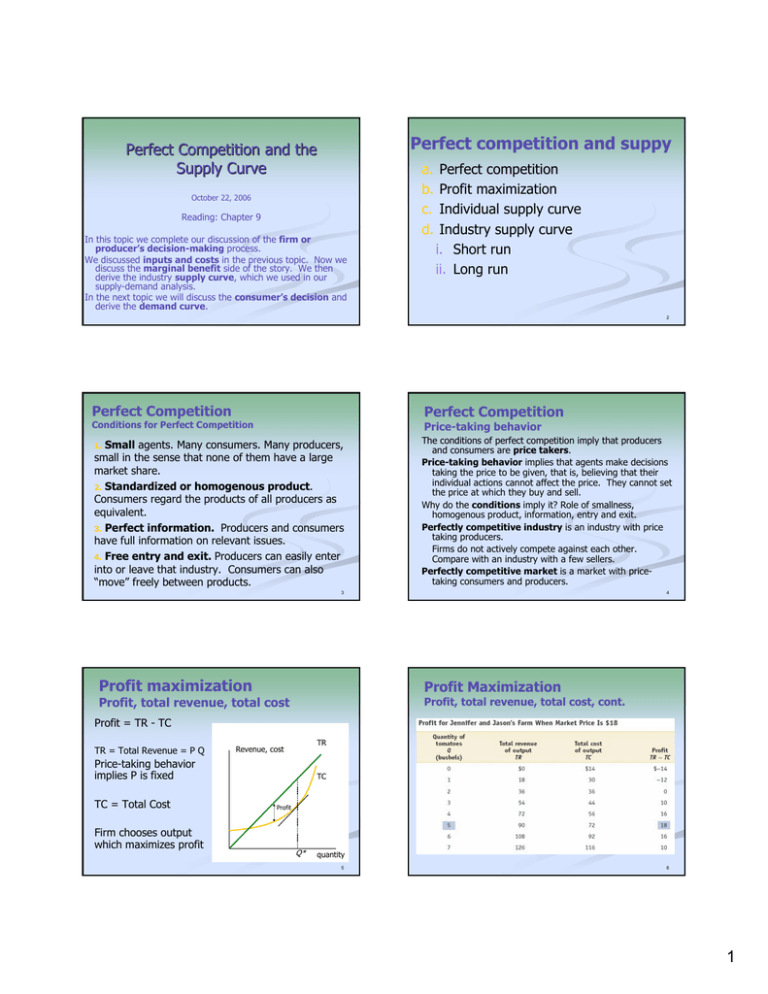
Perfect competition and suppy
Perfect Competition and the
Supply Curve
October 22, 2006
Reading: Chapter 9
In this topic we complete our discussion of the firm or
producer’s decision-making process.
We discussed inputs and costs in the previous topic. Now we
discuss the marginal benefit side of the story. We then
derive the industry supply curve, which we used in our
supply-demand analysis.
In the next topic we will discuss the consumer’s decision and
derive the demand curve.
a.
b.
c.
d.
Perfect competition
Profit maximization
Individual supply curve
Industry supply curve
i. Short run
ii. Long run
2
Perfect Competition
Perfect Competition
Conditions for Perfect Competition
Price-taking behavior
1. Small agents. Many consumers. Many producers,
small in the sense that none of them have a large
market share.
2. Standardized or homogenous product.
Consumers regard the products of all producers as
equivalent.
3. Perfect information. Producers and consumers
have full information on relevant issues.
4. Free entry and exit. Producers can easily enter
into or leave that industry. Consumers can also
“move” freely between products.
The conditions of perfect competition imply that producers
and consumers are price takers.
Price-taking behavior implies that agents make decisions
taking the price to be given, that is, believing that their
individual actions cannot affect the price. They cannot set
the price at which they buy and sell.
Why do the conditions imply it? Role of smallness,
homogenous product, information, entry and exit.
Perfectly competitive industry is an industry with price
taking producers.
Firms do not actively compete against each other.
Compare with an industry with a few sellers.
Perfectly competitive market is a market with pricetaking consumers and producers.
3
Profit maximization
4
Profit Maximization
Profit, total revenue, total cost, cont.
Profit, total revenue, total cost
Profit = TR - TC
TR = Total Revenue = P Q
TR
Revenue, cost
Price-taking behavior
implies P is fixed
TC = Total Cost
Firm chooses output
which maximizes profit
TC
Profit
Q*
quantity
5
6
1
Profit Maximization
Profit Maximization
Marginal Analysis
Marginal Analysis, cont
Marginal revenue is the change in total revenue
generated by an additional unit of output.
MR = ∆TR/∆Q
The optimal output rule says that profit is maximized by
producing the quantity of output at which the marginal cost of the
last unit produced is equal to its marginal revenue.
MR = MC
In a perfectly competitive industry: MR = P
Optimal output rule is: P = MC
7
Profit Maximization
8
Profit Maximization
Marginal Analysis, cont.
Profitable Production
Marginal
revenue curve
shows how
Marginal
Revenue
depends on the
level of output.
For perfect
competition, it is
given by price, P
The profit-maximizing point is where the marginal cost curve
crosses the marginal revenue curve (which is a horizontal line at
9
the market price).
Profit Maximization
Profitable Production, cont
¾ If TR > TC, the firm is profitable.
¾ If TR = TC, the firm breaks even.
¾ If TR < TC, the firm incurs a loss.
Profit/Q = TR/Q – TC/Q = P - AC
¾ If P > AC, the firm is profitable.
¾ If P = AC, the firm breaks even.
¾ If P < AC, the firm incurs a loss.
¾ Note: Cost include all opportunity costs
10
Profit Maximization
Profitable production, cont
The break-even price of a
price-taking firm is the market
price at which it earns zero
profits.
Profit making
Loss making
Whenever market price
exceeds minimum average
total cost, the producer is
profitable.
Whenever the market price
equals minimum average total
cost, the producer breaks
even.
Whenever market price is less
than minimum average total
cost, the producer is
11
unprofitable.
12
2
Individual Supply Curve
Individual Supply Curve
Firms output decision rules
Competitive Firm’s Profitability and Production Conditions
In the short run, fixed costs are given.
1. The firm will produce up to where P = MC, provided
MC is rising. When MC is falling, if output is
increased, TC falls and TR rises, so that profit
increases.
2. The firm will produce nothing if P < minimum AVC.
If firm produces nothing, its profit = - TFC
If it produces something its profit = TR – TC
= TR – TFC – TVC = (P – AVC) Q – TFC
„ In the long run, fixed costs can be changed and the
firm can enter or exit.
If P > minimum AC, firm will exist. Otherwise it will
close down.
„
13
Individual Supply Curve
Firm’s supply curve
14
Industry Supply Curve: Short run
The industry supply curve shows the relationship between the
price of a good and the total output of the industry as a whole.
Short run industry supply curve is the horizontal sum of the
individual supply curve of all firms in an industry, given the
number of firms and given each firm’s fixed cost.
P
P
Firm 1
A firm will cease production in the short-run if the market price falls below the
15
shut-down price, which is equal to minimum average variable cost.
Industry Supply Curve: Short run
The Short-Run Market Equilibrium
q
P
Firm 2
P
Industry
Firm 3
q
q
16
Quantity
Industry Supply Curve: Long Run
The Long-Run Market Equilibrium
In the long run firms can change fixed costs and they can enter and exit.
Already considered changing fixed costs – deal with LRAC, LRMC
Now consider entry and exit, ignoring changes in fixed costs.
There is a short-run market equilibrium when the quantity supplied equals
17
the quantity demanded, taking the number of producers as given.
A market is in long-run market equilibrium when the quantity supplied
equals the quantity demanded, given that sufficient time has elapsed for entry
18
into and exit from the industry to occur.
3
Industry Supply Curve: Long Run
The Effect of an Increase in Demand in the ShortRun and the Long-Run
Industry Supply Curve: Long Run
Comparing the Short-Run and Long-Run Industry
Supply Curves
„ The long-run industry
supply curve can be
completely flat.
It can also be upward
rising. Why?
„
„
Rising input prices
External technical
diseconomies: Costs of
firms rise when industry
output rises – pollution?
„
It can also be downward
sloping. Why? External
diseconomies.
„
D↑ Æ P↑ Æ non-zero profits Æ entry Æ S↑ Æ P↓ Æ back to zero profit
(on LRS curve)
19
The long-run industry supply curve is always flatter—more elastic—than the
20
short-run industry supply curve. This is because of entry and exit:
Industry Supply Curve: Long Run
Industry Supply Curve: Long Run
Negatively-sloped Long Run Supply Curve
Positively-sloped Long Run Supply Curve
Demand curve moves up. Price goes up along SRSC. Positive profits.
Firm enter. SRSC moves right and industry output expands. Pushes up
firm cost curves due to higher input prices or technological external
diseconomies. Long-run equilibrium price is higher than before.
Demand curve moves up. Price goes up along SRSC. Positive profits.
Firm enter. SRSC moves right and industry output expands. Pushes
down firm cost curves due to technological external economies. Longrun equilibrium price is lower than before.
price
price
ATC
MC
MC
D
SRSC
D
SRSC
ATC
LRSC
LRSC
quantity
quantity
Quantity
21
Quantity
22
Industry Supply Curve: Long Run
Implications of Long Run Equilibrium
1. In a perfectly competitive industry in equilibrium, the
value of marginal cost is the same for all firms.
2. In a perfectly competitive industry with free entry and
exit, each firm will have zero economic profits in longrun equilibrium.
23
4