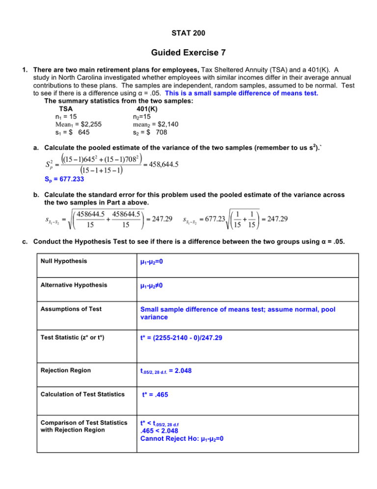
STAT 200
Guided Exercise 7
1. There are two main retirement plans for employees, Tax Sheltered Annuity (TSA) and a 401(K). A
study in North Carolina investigated whether employees with similar incomes differ in their average annual
contributions to these plans. The samples are independent, random samples, assumed to be normal. Test
to see if there is a difference using α = .05. This is a small sample difference of means test.
The summary statistics from the two samples:
TSA
401(K)
n1 = 15
n2=15
Mean1 = $2,255
mean2 = $2,140
s1 = $ 645
s2 = $ 708
a. Calculate the pooled estimate of the variance of the two samples (remember to us s2).`
S p2 =
((15 −1)645
2
)
+ (15 − 1)7082
= 458,644.5
(15 − 1 + 15 − 1)
Sp = 677.233
b. Calculate the standard error for this problem used the pooled estimate of the variance across
the two samples in Part a above.
⎛ 458644.5 458644.5 ⎞
sx1 −x2 = ⎜
+
⎟ = 247.29
15
⎝ 15
⎠
⎛ 1 1 ⎞
sx1 −x2 = 677.23 ⎜ + ⎟ = 247.29
⎝ 15 15 ⎠
c. Conduct the Hypothesis Test to see if there is a difference between the two groups using α = .05.
Null Hypothesis
µ1-µ2=0
Alternative Hypothesis
µ1-µ2≠0
Assumptions of Test
Small sample difference of means test; assume normal, pool
variance
Test Statistic (z* or t*)
t* = (2255-2140 - 0)/247.29
Rejection Region
t.05/2, 28 d.f. = 2.048
Calculation of Test Statistics
Comparison of Test Statistics
with Rejection Region
t* = .465
t* < t.05/2, 28 d.f
.465 < 2.048
Cannot Reject Ho: µ1-µ2=0
d. Confirm that if the sample sizes are equal for each group, the pooled variance is simply the average
of the two variances.
(416,025+501,264)/2 = 458,644.5
When the two sample sizes are equal, the pooled variance formula simplifies to an average of the
variances.
2. Geneticists have identified E2F1 transcription factor as an important component of cell
proliferation control. The researchers induced DNA synthesis in two batches of serum-starved cells.
In one group of 92 cells (treatment), cells were micro-injected with the E2F1 gene. A control group of
158 cells was not exposed to E2F1. After 30 hours, researchers determined the number of altered
growth cells in each batch. Test to see if the proportion of growth altered cells for the treatment group is
larger than that of the control. Conduct the hypothesis test using Use α = .01.
Note: this is a difference of proportions test. For a difference in proportions test where the null
hypothesis says the two groups are equal, we should make a pooled estimate of the proportion (using
information from both groups) to estimate the standard error of our test.
Control
E2F1 Treated
Pooled estimate
Total cells
158
92
250
Number of growth altered cells
15
41
56
p for each group
a.
.0949
.4457
.2240
The pooled estimate of p for this problem is (denoted as pp) and the pooled estimate
of q (denoted as qp) :
pp =
b.
(15 + 41) = 56 = .2240
(158 + 92) 250
The standard error for this test is (note the formula to the right): σ ( p1 − p2 ) =

&1 1#
p p q p $$ + !!
% n1 n2 "
⎛ 1 1 ⎞
1 ⎞
⎛ 1
+ ⎟⎟ = .2240 * .7760⎜
+ ⎟ = .0547
⎝ 158 92 ⎠
⎝ n1 n2 ⎠
σ ( p − p ) = p p q p ⎜⎜
1
c.
2
Conduct the Hypothesis Test to see if the proportion of growth altered cells for the treatment
group is larger than that of the control. Conduct the hypothesis test using Use α= .01.
Null Hypothesis
Pt - Pc = 0
Alternative Hypothesis
Pt - Pc > 0 one-tailed test
Assumptions of Test
Large sample difference of proportions test; assume normal, pool
variance
Test Statistic (z* or t*)
z* = (.4457-.0949 - 0)/.0547
Rejection Region
z.01 = 2.33
Calculation of Test Statistic
z* = 6.42
Comparison of Test
Statistics with Rejection
Region
z* > z.01 6.42 > 2.33
Reject Ho: Pt - Pc = 0
d.
What is the p-value for the test statistic?
A z* = 6.42 is very large.
We can’t even look it up in the standard normal
table
So just say, p < .001
This is very small and good enough for most
people reading your research
By the way, the real p is .0000000001!
Females
Males
About Right
87
64
151
Overweight
39
3
42
3
26
29
Underweight
Column Totals
129
93
Row Total
222
3. The following is some data from a survey of 222 college students. The data show the breakdown
of responses to how they feel about their weight by their gender. The responses to how they perceived
their own weight were, “about right,” “overweight,” and “underweight.” The data are given to the right. We
can assume that their feelings about their weight is the “dependent” variable.
a. We will focus on the Female vs Male response to “About Right.” I want you to conduct a difference of
proportion test to determine if Females and Males had different perceptions about their weight being
“About Right.” Use alpha = .05.
Remember to calculate the pooled proportion for this problem first, before calculating the standard
error. Use alpha = .05

⎛ 1 1 ⎞
1 ⎞
⎛ 1
+ ⎟⎟ = .6802 * .3198⎜ +
⎟ = .0634
⎝ 93 129 ⎠
⎝ n1 n2 ⎠
σ ( p − p ) = p p q p ⎜⎜
1
2
pp = (87 + 64)/(129+93) = (151)/222 = .6802
HYPOTHESIS TEST
Null Hypothesis
Pm - Pf = 0
Alternative Hypothesis
Pm - Pf ≠ 0 two-tailed test
Assumptions of Test
Large sample difference of proportions test; assume normal, pool
variance
Test Statistic (z* or t*)
z* = (.6882-.6744 - 0)/.0634
Rejection Region
z.05. = 1.96
Calculation of Test Statistic
z* = .2177
Comparison of Test
Statistics with Rejection
Region
z* < z.05
.2177 < 1.96
Cannot reject Ho: Pm - Pf = 0
What is the p-value of your test?
The p-value? Look up .22 in standard normal table. .0871
Subtract from .5 .5-.0871 = .4129
Multiply by 2 for two-tailed test .8258
4. This problem looks at the salary differences of Male and Female Mid-Level Managers at 220 firms.
We will be looking at an Excel file with data on mid-level managers in 220 firms. The salary is given in
$1,000s. We want to look at the female sample (n=75) and compare it to the male mean level (144) to
see if it is lower than that of males (or if males is higher). Use an alpha level of .01.
Here are the Excel output:
a. Summarize the salary levels for men and women at the company using the descriptive statistics.
Male salary slightly larger – $144K compared to $140k for females.
Mean and median very close for both groups.
Variances are very similar for both groups
Spread is not too large for either group – they are all managers approximately 8.8% C.V.
Here is the JMP output for a t-test assuming unequal variances. Use it to conduct the test below using
an alpha level of .01.
c. Conduct the Hypothesis Test to see if women earn less than men using α = .01.
Null Hypothesis
µm-µf=0
Alternative Hypothesis
µm-µf≠0
Assumptions of Test
Large sample difference of means test; assume normal, pool
variance
Test Statistic (z* or t*)
t* = 2.056
Critical Value at the Rejection
Region
t = 2.352
Comparison of Test Statistics
with Rejection Region
The test statistics is 2.056 it is less that the critical value at the
rejection region. We cannot reject Ho: No difference
d. What is the p-value for this test?
All we need do is read the value from the JMP output. Given this is a two-tailed test we use
Prob > |t| = .0415
e. How would you explain your test result in words.
We observed a difference between of the male and female salary of $3,644. When we tested that
difference it was not statistically significant at the .01 level for a two-tailed test. This at this level of
certainty we cannot be sure if there is a real difference. However, our test would have been significant
it the error rate was .05, since the p-value for a two-tailed test was .0415.
f.
Could we have assumed the variances of the two groups were equal? Brainstorm a bit to decide
how we might do this?
The easiest way to do this is to divide the two variances and see if the result is close to one. In a
formal test, this is called an F-test and it follows an F-distribution. When creating this ratio it is best to
put the larger variance first, so we will look at the rtion of females to males. For our purposes the ratio
is:
156.144/153.613 = 1.016
These variances are very close to one another and it would have been reasonable to assume the
variances were equal. In terms of our test, this would have changed the standard error a small bit, and
the degrees of freedom would have increased from 148.687 to (145-1) + (75-1) = 218. However, using a
pooled variance would not have changed the result of the test at alpha = .01 level.
g. I am including the output assuming equal variances from JMP. Did it change the results of the test
much?
Very little difference
whether we assume or not
assume equal variances –
the sample sizes are
LARGE
4. Earlier we look at some summary data from each state and the District of Columbia for a 20
question test on driving. The score of the test was calculated as 5 points for each correct question. I
administered the same test to 65 graduate and undergraduate students in statistic classes in summer
2010. I am going to give you the summary information on the scores for all 65 students as well as a
breakdown of the scores for graduate students and undergraduate students from JMP. I want you to do
the following:
a. Describe the distribution of the test for all 65 students.
b. Conduct a two-tailed difference of means test between undergraduate and graduate students. The
results are given in JMP. All you need to do is summarize the results.
H0: µundergrad – µgrad = 0
Ha: µundergrad – µgrad NE 0 two-tailed test
Assume equal variances.
The test statistic from JMP is -1.960 The p-value for a two-tailed test for this value is .0545. This result
would not meet the criteria for a two-tailed test with alpha equal to .05. It would meet the criteria is we
were able to accdept a larger Type I error, for example at alpha equal to .10.
Based on an alpha level of .05, we would fail to reject the Null Hypothesis and conclude we do not have
enough evidence to say the scores of undergrads and graduate students are different.
c. Would the results have mattered if we used a one-tailed test that graduate students would score better
than undergraduate students?
If we used a one-tailed test the p-value is .0272 that undergraduate students are lower than graduate
students (this means the same thing as graduate students score better). Note the JMP software conducted
the test as Undergraduate – Graduate. Based on this result, we would have been able to reject at alpha
equal to .05.