Be Mean Green!
Please consider the environment before printing this Chapter Outline. It’ll be available online throughout the semester.
Aggregate Demand- Aggregate Supply Model (AD-AS Model) – a macroeconomic model that uses aggregate demand and aggregate supply to determine and explain the price level and level of real domestic output.
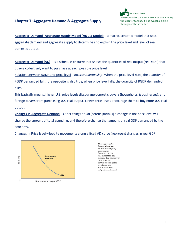
Aggregate Demand (AD) – is a schedule or curve that shows the quantities of real output (real GDP) that buyers collectively want to purchase at each possible price level.
Relation between RGDP and price level – inverse relationship : When the price level rises, the quantity of
RGDP demanded falls; the opposite is also true, when price level falls, the quantity of RGDP demanded rises.
This basically means, higher U.S. price levels discourage domestic buyers (households & businesses), and foreign buyers from purchasing U.S. real output. Lower price levels encourage them to buy more U.S. real output.
Changes in Aggregate Demand – Other things equal (ceteris paribus) a change in the price level will change the amount of total spending, and therefore change that amount of real GDP demanded by the economy.
Changes in Price level – lead to movements along a fixed AD curve (represent changes in real GDP).
1

Changes in the Determinants of AD – lead to a shifting of the AD curve (i.e., the entire AD curve will shift)
The Determinants of AD are:
1.
Change in Consumer spending (C) a.
Consumer wealth – Consumer wealth is the total dollar value of assets (ex: stocks, bonds, real estate, etc.), minus the dollar value of liabilities or debts (ex: mortgages, car loans, credit card balances, etc.).
Consumer wealth sometimes changes suddenly and unexpectedly, due to unexpected changes in asset values. (ex: sudden increase in stock values, real estate values, etc. ) This gives consumers more spending power, making the AD curve to shift to the right – “wealth effect”. The opposite can happen, for example, with a stock market crash, real estate values dropping, etc., can lead to a “reverse wealth effect” and cut consumer spending drastically, increase saving, thus shifting the AD curve to the left. b.
Household borrowing – Consumers can increase their consumption spending by borrowing, shifting the AD curve to the right. Decrease in borrowing, shifts the AD curve to the left. c.
Consumer expectations – changes in expectations about the future may alter consumer spending d.
Personal taxes – A reduction in personal income tax rates raises take-home pay, and increases consumer spending at each possible price level – AD Curve shifts to the right. Higher personal taxes reduce consumption, shifting the AD curve to the left.
2.
Change in Investment spending (I) a.
Interest rates – real interest rates b.
Expected returns
- Expected future business conditions
- Technology
- Degree of excess capacity
- Business taxes
3.
Change in Government spending (G) – An increase in government spending shifts the AD curve to the right. The opposite is also true.
4.
Change in Net Export spending (NX) a.
National income abroad – Rising national income abroad encourages foreigners to buy more products, some of which are made in the U.S. So, U.S. net exports rise, and the U.S. AD Curve
2

shifts to the right. Declines in national income abroad has the opposite effect, shifting the U.S.
AD curve to the left. b.
Exchange rates – related to the appreciation or depreciation of the dollar. For example dollar depreciation increases net exports, imports go down and exports go up. The opposite is also true.
3

Aggregate Supply (AS) – is a schedule or curve showing the relationship between the price level, and the amount of real domestic output (real GDP) that firms in the economy produce. This relationship varies depending on the time horizon and how quickly output prices and input prices change.
The three time horizons are:
In the immediate short run, both input and output prices are fixed.
In the short run, input prices are fixed, but output prices can vary.
In the long run, input and output prices can vary.
Immediate short run AS Curve:
Short run AS curve : Long run AS curve:
Even though each of these scenarios for AS: immediate short run, short run and long run, are all important for appropriate for analysis of different situations, we will look at the short-run aggregate supply curve (AS Curve), the second one in the above set of AS curves. This is to help us understand the business cycle in a simple way.
Changes in Aggregate Supply
Changes in Price level – input prices are sticky (fixed), output prices can change. This leads to movements along a fixed AS curve (represent changes in real firm profits).
Changes in the Determinants of AS – lead to a shifting of the AS curve (i.e., the entire AS curve will shift)
The Determinants of AS are:
1.
Change in input prices a.
Domestic resource prices b.
Imported resource prices
4

2.
Change in productivity:
Productivity=
Total output
Total inputs
3.
Change in legal-institutional environment a.
Business taxes b.
Government regulations
Equilibrium Price Level and Real GDP
Question: Of all the possible combinations of price levels and levels of real GDP, which combination will the economy generate?
Answer: Equilibrium occurs at the price level that equalizes the amounts of real output demanded and supplied. The intersection of AD and AS curves establishes the equilibrium price level and equilibrium real output (real GDP).
So, AD and AS jointly establish the price level and level of real GDP.
Changes in the Price level and Real GDP
AD and AS typically change from one period to the next.
Demand-Pull inflation Cost-Push inflation
5

Recession and Cyclical unemployment
Here the price level is not changing even though AD has decreased (downward price-level inflexibility – sticky prices). Since, AS also is less, fewer people are needed to produce the required output and in this recessionary scenario, Cyclical unemployment rises.
The reasons for downward price-level inflexibility are as follows:
- Fear of price wars
- Menu costs
- Wage contracts
- Morale, effort, and productivity
- Minimum wage
Recessions usually prompt the government and the Federal Reserve to take actions to try to increase
Aggregate Demand (AD).
The Multiplier Effect
Change in Real GDP
Multiplier =
Initial change in spending
By rearranging the above equation, we get
Change in Real GDP = Multiplier x Initial change in spending.
6