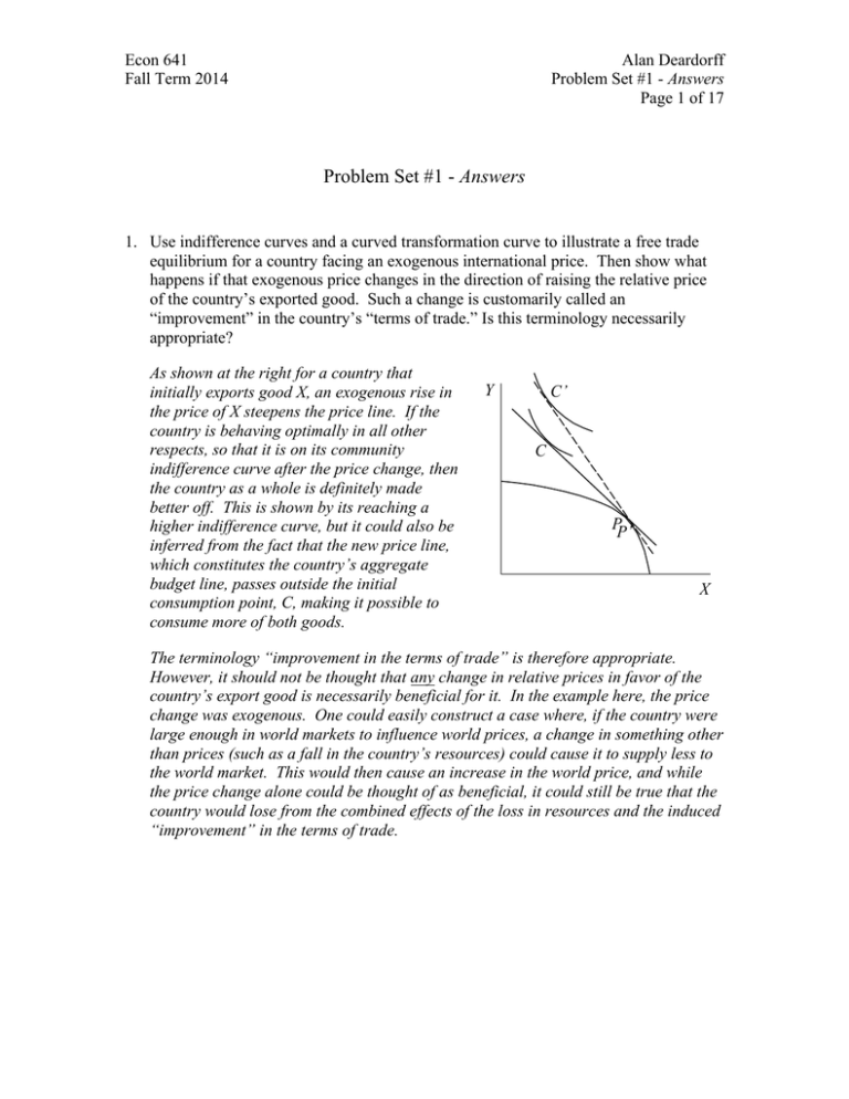
Econ 641
Fall Term 2014
Alan Deardorff
Problem Set #1 - Answers
Page 1 of 17
Problem Set #1 - Answers
1. Use indifference curves and a curved transformation curve to illustrate a free trade
equilibrium for a country facing an exogenous international price. Then show what
happens if that exogenous price changes in the direction of raising the relative price
of the country’s exported good. Such a change is customarily called an
“improvement” in the country’s “terms of trade.” Is this terminology necessarily
appropriate?
As shown at the right for a country that
initially exports good X, an exogenous rise in
the price of X steepens the price line. If the
country is behaving optimally in all other
respects, so that it is on its community
indifference curve after the price change, then
the country as a whole is definitely made
better off. This is shown by its reaching a
higher indifference curve, but it could also be
inferred from the fact that the new price line,
which constitutes the country’s aggregate
budget line, passes outside the initial
consumption point, C, making it possible to
consume more of both goods.
Y
C’
C
PP’
X
The terminology “improvement in the terms of trade” is therefore appropriate.
However, it should not be thought that any change in relative prices in favor of the
country’s export good is necessarily beneficial for it. In the example here, the price
change was exogenous. One could easily construct a case where, if the country were
large enough in world markets to influence world prices, a change in something other
than prices (such as a fall in the country’s resources) could cause it to supply less to
the world market. This would then cause an increase in the world price, and while
the price change alone could be thought of as beneficial, it could still be true that the
country would lose from the combined effects of the loss in resources and the induced
“improvement” in the terms of trade.
Econ 641
Fall Term 2014
Alan Deardorff
Problem Set #1 - Answers
Page 2 of 17
2. The diagram below shows a free-trade equilibrium between two countries, A and B.
Technological change now causes country A to be able to produce exactly 10% more
output of good X than it could before, for any given input of resources.
a) Determine what this will do to the two countries’ transformation curves, to their
offer curves, and therefore to the world equilibrium prices.
The change in technology does nothing to
Country B’s transformation curve, but it
stretches A’s to the right by 10%, as shown
in the broken curve at the right. (The shift
shown is somewhat more than 10%, to make
it easier to see.) At initial prices (shown by
the parallel price line tangent to the new
transformation curve), output of X rises and
output of Y falls (since the expansion
flattens the transformation curve by 10% at
the point where Y is unchanged).
Consumption moves to the new tangency of
the price line with an indifference curve, but
without assumptions about preferences this
could entail a fall in demand for one of the
goods if it is an inferior good. The case
shown has demand rising for both, in which
case desired trade expands, since production
of Y falls while consumption of Y rises. In
general, if good Y is sufficiently inferior, its
consumption could fall by more than
production and desired trade would
contract.
Country A
Y
p0
p0
X
Y
A’
p0
p1
A
B
What happens to the offer curves can be
inferred from this change in trade at
constant prices. Country B’s offer curve is
X
unchanged, while Country A’s expands
outward from the origin if good Y is a normal good, as drawn, but could contract
inward if Y is sufficiently inferior.
This in turn causes the world price of good X to change, falling in the case shown
of Y a normal good, but possibly rising if Y is sufficiently inferior for the A offer
curve to contract.
Econ 641
Fall Term 2014
Alan Deardorff
Problem Set #1 - Answers
Page 3 of 17
b) Without further assumptions about preferences, are there any of these variables
the direction of change in which cannot be determined unambiguously?
As already indicated, the direction of shift of country A’s offer curve is
ambiguous, as is therefore the direction of change in the world relative price.
c) If you assume that preferences are homothetic, can any of these ambiguities be
resolved?
Yes. With homothetic preferences (or even just with good Y a normal good, which
is weaker than homotheticity), country A’s offer curve must expand as shown and
the world relative price of A’s export good, X, must fall.
d) Show the new equilibrium in both countries for the case of homothetic
preferences.
Country A
Y
Country B
Y
X
X
Since we know that the world price of X falls, we can be sure that country B’s
output of X falls and its consumption of both goods rises (again, due to
homotheticity). Thus B’s imports of X must rise, although its exports of Y may
rise or fall. The case drawn has Country A still reaching a higher indifference
curve than it did before the expansion, but this is not necessary. Country A could
lose from its own expansion, the case of Bhagwati’s “Immizerizing growth.” (See
Bhagwati, Jagdish. 1958. "Immiserizing Growth: A Geometrical Note," Review
of Economic Studies 25, (June), pp. 201-205.)
Econ 641
Fall Term 2014
3.
Alan Deardorff
Problem Set #1 - Answers
Page 4 of 17
Consider a country engaged in production and trade of an arbitrary number of goods.
Assume that there are no transport costs and that producers are competitive profit
maximizers. Assuming that trade is free, show that if the vector of world prices, pw,
changes by a vector Δpw, then the vector of the resulting changes in outputs, ΔX, will
be nonnegatively correlated with Δpw (assuming that pw is always normalized to lie on
the unit simplex).
From maximization
p0w X 0 ≥ p0w X ∀X ∈ F
and similarly
p1w X 1 ≥ p1w X ∀X ∈ F
where
p1w = p0w + Δ p w
1
0
X = X + ΔX
Letting X = X 1 in the first inequality and X = X 0 in the second, we can add them
together to get
p0w X 0 + p1w X 1 ≥ p0w X 1 + p1w X 0
or
p0w ( X 0 - X 1) + p1w ( X 1 - X 0 ) ≥ 0
(p1w - p0w )( X 1 - X 0 ) ≥ 0
Δ p wΔX ≥ 0
If p0w and p1w are both on the unit simplex (which means that the elements of both
vectors add up to one), then the sample mean of the elements in Δ p w is
Econ 641
Fall Term 2014
Alan Deardorff
Problem Set #1 - Answers
Page 5 of 17
1
Mean(Δ p w ) = ∑Δ p wj
n
1
= ∑(p1wj - p0wj)
n
1
= #$∑ p1wj - ∑ p0wj%&
n
1
= [1 - 1] = 0
n
Therefore the correlation between Δ p w , and ΔX has the same sign as their inner
product:
Sign[Cor(Δ p w,ΔX)] = Sign[Δ p wΔX] ≥ 0
(See Deardorff, “The Correlation Between Price and Output Changes When
There Are Many Goods,” Journal of International Economics 10, August 1980,
pp. 441-43.)
4. a) Derive and draw the transformation curves of the two economies whose
endowments and technologies are those described below. Each has a fixed
endowment of labor – its only factor of production – and can produce two goods,
X and Y, using the following constant amounts of labor per unit of output:
Per-unit labor requirement
for producing
Endowment
of Labor
X
Y
Country A
60
1
2
Country B
120
2
3
Econ 641
Fall Term 2014
Alan Deardorff
Problem Set #1 - Answers
Page 6 of 17
Country A
Country B
Y
Y
40
30
60
X
60
X
b) How much of goods X and Y will be produced and consumed in autarky in these
two countries, and what will be their relative prices, assuming that demanders
always insist on consuming them in fixed proportions of 1 unit of X for each unit
of Y?
A:
X=Y
X + 2Y = 60
3X = 60
X = Y = 20
pX /pY = 2
B:
X =Y
2X + 3Y = 120
5X = 120
X = Y = 24
pX/pY = 2/3
c) Derive and draw the world transformation curve.
Econ 641
Fall Term 2014
Alan Deardorff
Problem Set #1 - Answers
Page 7 of 17
Y
Y=X
70
60
40
60
120
X
d) Derive the free trade equilibrium relative price of X and Y, plus the equilibrium
quantities of the goods produced, consumed, and traded.
From the picture in part (c), Y=X requires producing in the upper segment of the
world transformation curve. Thus with free trade
pX 1
=
pY 2
and outputs in country B are
B
B
X = 0, Y = 40
World outputs:
W
W
A
A
X = Y = X = Y + 40
A
A
X + 2Y = 60
W
W
X + 2( X - 40) = 60
3 X W = 60 + 80 = 140
140
2
W
W
= 46
X =Y =
3
3
2
2
2
∴ X A = 46 , Y A = 46 -40 = 6
3
3
3
A’s income in units of Y = 30:
1 A
A
A
A
X = Y , X + Y = 30
2
3 A
2
A
A
X = 30, X = 30 = 20, Y = 30 - 10 = 20
2
3
∴ X A = Y A = 20
B’s income in units of Y = 40:
Econ 641
Fall Term 2014
Alan Deardorff
Problem Set #1 - Answers
Page 8 of 17
1 B
B
X + Y = 40
2
3 B
2
2
B
B
X = 40, X = 40 = 26 = Y
2
3
3
2
∴ X B = Y B = 26
3
B
B
X =Y ,
Trade:
2
units of X.
3
1
B exports 13 of Y.
3
A exports 26
5. In the Dornbusch, Fischer, and Samuelson Ricardian model with transport costs,
suppose that there is an increase in the cost of transportation, and suppose also that
other conditions happen to be such that the wage ratio, ω, remains unchanged as a
result. Determine the effects of this change on
a) the pattern of trade and specialization (which goods each country produces,
exports, and imports,
b) the domestic prices of goods in both countries, and
c) real wages (the ratio of the wage to an arbitrary index of domestic prices). Hint:
for the real wage, see if you can show that the nominal wage either rises or falls
relative to the prices of all goods. If so, then the exact price index does not
matter.
Econ 641
Fall Term 2014
Alan Deardorff
Problem Set #1 - Answers
Page 9 of 17
The initial equilibrium is shown below by the solid curves for gA, (1/g)A, and the
associated zA and zB. The initial wage ratio is ω0, with A producing [0,zA) and B
producing (zB,1]. A exports [0,zB), B exports (zA,1], and (zB,zA) are not traded.
(1 / g ʹ′) A
(1 / g) A
gA
g ʹ′A
ω0
0
z ʹ′B
zB
zA
z ʹ′A
1
a.
When the cost of transportation increases, the fraction of each
good that survives being traded, g, falls from g to g′. The curves shift to the
positions shown by the dashed curves g′A and (1–g′)A. Each country now
produces a larger range of goods, [0,z′A) and (z′B,1] respectively, while each
country exports a smaller range of goods, [0,z′B) and (z′A,1].
b.
With nominal wages unchanged, the prices of domestically
produced goods in each country are unchanged, while the prices of goods that
continue to be imported rise by the increase in transport costs. The prices of
goods that were previously imported but no longer are also rise but by less than
the increase in transport costs.
c.
Since nominal wages are unchanged, and since all prices in each
country either remain unchanged or rise, the real wage in each country falls.
Econ 641
Fall Term 2014
Alan Deardorff
Problem Set #1 - Answers
Page 10 of 17
6. In the Edgeworth Box below, point E is one point on the efficiency locus for the two
industries, X and Y, whose representative isoquants are as shown. Assuming that the
production functions for X and Y are linearly homogeneous, derive the rest of the
efficiency locus.
OY
E
X=X0
T
Y=Y0
OX
L
OY
B
E
A
X=X0
T
Y=Y0
OX
L
Ans: By expanding and contracting the two isoquants radially with respect to their
origins, you can find other points on the efficiency locus. Note that the resulting
locus, OXAEBOY, is not concave to the diagonal. You should check, however, that the
resulting transformation curve, though piecewise linear, is concave to its origin.
Econ 641
Fall Term 2014
Alan Deardorff
Problem Set #1 - Answers
Page 11 of 17
7. The following are the equations used by Jones (1965) to determine factor-price
changes from commodity-price changes:
θ LX wˆ + θTX rˆ = pˆ X
θ LY wˆ + θTY rˆ = pˆ Y
where θ Li + θTi = 1 , i = X, Y. Solve these equations for ŵ and r̂ in terms of pˆ X and
pˆ Y . From your solution, show that if good X is relatively labor intensive, so that
θ LX > θ LY , then a rise in p X relative to pY will raise w relative to both prices and
reduce r relative to both prices.
Ans:
wˆ =
pˆ X
pˆ Y
θ LX
θ LY
θ TX
θ TY
θ pˆ − θ TX pˆ Y
θ TY pˆ X − θ TX pˆ Y
= TY X
=
θ TX θ LX θ TY − θ LY θ TX θ LX (1 − θ LY ) − θ LY (1 − θ LX )
θ TY
θ TY pˆ X − θ TX pˆ Y (θ TY − θ TX ) pˆ X + θ TX ( pˆ X − pˆ Y )
=
θ LX − θ LY
θ LX − θ LY
θ TX
( pˆ X − pˆ Y )
= pˆ X +
θ LX − θ LY
=
(1)
θ TY ( pˆ X − pˆ Y ) + (θ TY − θ TX ) pˆ Y
θ TY − θ TX
θ TY
( pˆ X − pˆ Y ) + pˆ Y
=
θ TY − θ TX
(2)
or
wˆ =
If pˆ X − pˆ Y > 0 and θ LX > θ LY (and hence θTY > θTX ) , then
From (1): w
ˆ > pˆ X
From (2): w
ˆ > pˆ Y
Similarly
θ LX
θ
rˆ = LY
θ LX
θ LY
= pˆ Y −
pˆ X
pˆ Y
θ TX
θ TY
=
θ LX pˆ Y − θ LY pˆ X (θ LX − θ LY ) pˆ Y − θ LY ( pˆ X − pˆ Y )
=
θ LX − θ LY
θ LX − θ LY
θ LY
( pˆ X − pˆ Y )
θ LX − θ LY
(3)
Econ 641
Fall Term 2014
Alan Deardorff
Problem Set #1 - Answers
Page 12 of 17
or
θ LX ( pˆ Y − pˆ X ) + (θ LX − θ LY ) pˆ X
θ LX − θ LY
− θ LX
( pˆ X − pˆ Y ) + pˆ X
=
θ LX − θ LY
rˆ =
(4)
If pˆ X − pˆ Y > 0 and θ LX > θ LY , then
From (3): rˆ < pˆ Y
From (4): rˆ < pˆ X
8. Use the Lerner (unit-value-isoquant) diagram to work out the effects of a price
change in the 2×2 Heckscher-Ohlin model as follows. Consider a small country that
faces prices p 0x and p 0y for goods X and Y. Suppose that its endowments of labor
and land are such that, at these prices, it produces exactly $2 worth of each good.
Work out what happens when the price of good X rises by 20%, to p1x , the price of
good Y remaining constant. Assume that good X is the relatively labor-intensive
good. Determine, if possible, the direction of change in the following variables:
i)
The nominal wage.
ii)
The ratio of the nominal wage to the price of good X.
iii)
The rental price of land.
iv)
The ratio of land to labor used in producing good X.
v)
The ratio of land to labor used in producing good Y.
vi)
The average ratio of land to labor employed in both industries
together.
vii)
The output of good X.
viii)
The output of good Y.
Econ 641
Fall Term 2014
Alan Deardorff
Problem Set #1 - Answers
Page 13 of 17
Ans: First draw the Lerner diagram for the initial situation.(Draw it big enough to see
what’s going on.)
T
t
(L ,T )
0
Y
Y 0 = 2 / pY0
t X0
Y = 1 / pY0
X 0 = 2 / p X0
X = 1 / p X0
O
L
Econ 641
Fall Term 2014
Alan Deardorff
Problem Set #1 - Answers
Page 14 of 17
Now construct the new equilibrium with the price of X 20% higher: p1X = 1.2 p X0 . This
shifts the unit-value X-isoquant approximately 20% in toward the origin (actually by 1/6,
though I’ve drawn it shifting more, for clarity). From that construct the new common
tangent, the rays for t 1X and tY1 , and the parallelogram showing the allocation of factors
that will maintain full employment of each. Isoquants through these allocations indicate
the new outputs X1 and Y1.
T
tY1
(L ,T )
t
0
Y
Y 0 = 2 / pY0
Y1
t1X
Y = 1 / pY0
t X0
X1
X 0 = 2 / p X0
X = 1 / p X0
X = 1 / p1X
O
L
From this figure you can read the results for parts (iv)-(viii). The ratio of land to labor
has increased in both industries, although the average ratio of land to labor employed
has not changed (since it must continue to equal the unchanged endowment). That is
possible because more of both factors is employed in the X industry and less of both in
the Y industry, resulting in a larger output of X and a smaller output of Y.
Econ 641
Fall Term 2014
Alan Deardorff
Problem Set #1 - Answers
Page 15 of 17
To get effects on factor prices, use the intercepts of the isocost lines to measure their
reciprocals in nominal terms – that is, in units of the currency in which the prices have
been expressed. From these it follows immediately that the nominal wage has risen and
the nominal rental on land has fallen. This is also a fall in the real rental, since one
price is unchanged and the other has risen.
T
tY1
(L ,T )
t
0
Y
Y 0 = 2 / pY0
Y1
1/r
1
t1X
X1
0
Y
Y = 1/ p
t X0
1/r0
X 0 = 2 / p X0
X = 1 / p X0
X = 1 / p1X
O
1/w1
1/w~
1/w0
L
To find the effect on the real wage, construct a wage, w~, which is above w0 by just the
percentage of the price increase. This is done by constructing the dotted line parallel to
the initial isocost line but tangent to the new unit-value X-isoquant. It is then clear that
the new wage, w1is above w~ and has therefore risen not only relative to the constant
price of Y but relative also to the increased price of X. Thus the real wage of labor is
increased.
Econ 641
Fall Term 2014
Alan Deardorff
Problem Set #1 - Answers
Page 16 of 17
9. The Lerner diagram below shows an initial equilibrium, in the 2×2 Heckscher-Ohlin
model, for a small-open economy facing fixed world prices of goods X and Y, p 0X
and pY0 . Its initial endowments of the two factors, unskilled labor U and skilled labor
S, are shown by point E. Suppose now that some unskilled workers become skilled,
moving the endowment point first to E’ and then to E’’. Determine the effects of
these changes on outputs of both goods and on factor prices.
S
E′′
E′
E
Y = 1 / pY0
X = 1 / p X0
O
U
S
tY1
tY0
E′′
Y2
1/s2
1/s0
Y = 1 / pY0
E
Y0
X2=0
O
E′
Y1
X1
t X0
X0
X = 1 / p X0
1/w2
1/w0
U
Econ 641
Fall Term 2014
Alan Deardorff
Problem Set #1 - Answers
Page 17 of 17
Constructing parallelograms from points E and E′, this initial allocation and the
allocation for endowment E′ are both found inside the diversification cone, i.e., between
rays t X0 and tY0 . For endowment E′′, since it is outside the cone, only good Y is produced
using the expanded version of the Y isoquant through E′′. Using the distance from the
origin along rays t X0 and tY0 to measure output, one sees that output of X falls from X0 to
X1 and then to X2=0. Output of Y rises from Y0 to Y1 to Y2.
The wage of unskilled labor, w, is initially w0 and remains there when the endowment
moves to E′. But when the endowment moves outside the cone to E′′, then the unskilled
wage rises to w2. Likewise, the wage of skilled labor, s, remains at s0 for E and E′, but
then falls to s2 at E′′.