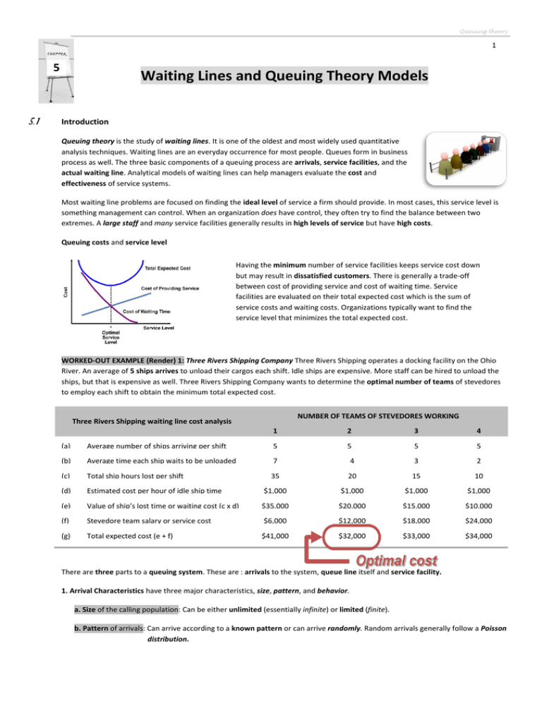
Queuing theory
1
5
5.1
Waiting Lines and Queuing Theory Models
Introduction
Queuing theory is the study of waiting lines. It is one of the oldest and most widely used quantitative
analysis techniques. Waiting lines are an everyday occurrence for most people. Queues form in business
process as well. The three basic components of a queuing process are arrivals, service facilities, and the
actual waiting line. Analytical models of waiting lines can help managers evaluate the cost and
effectiveness of service systems.
Most waiting line problems are focused on finding the ideal level of service a firm should provide. In most cases, this service level is
something management can control. When an organization does have control, they often try to find the balance between two
extremes. A large staff and many service facilities generally results in high levels of service but have high costs.
Queuing costs and service level
Having the minimum number of service facilities keeps service cost down
but may result in dissatisfied customers. There is generally a trade-off
between cost of providing service and cost of waiting time. Service
facilities are evaluated on their total expected cost which is the sum of
service costs and waiting costs. Organizations typically want to find the
service level that minimizes the total expected cost.
WORKED-OUT EXAMPLE (Render) 1: Three Rivers Shipping Company Three Rivers Shipping operates a docking facility on the Ohio
River. An average of 5 ships arrives to unload their cargos each shift. Idle ships are expensive. More staff can be hired to unload the
ships, but that is expensive as well. Three Rivers Shipping Company wants to determine the optimal number of teams of stevedores
to employ each shift to obtain the minimum total expected cost.
NUMBER OF TEAMS OF STEVEDORES WORKING
Three Rivers Shipping waiting line cost analysis
1
2
3
4
5
5
5
(a)
Average number of ships arriving per shift
5
(b)
7
4
3
2
35
20
15
10
(d)
Average time each ship waits to be unloaded
(hours)
Total ship hours lost per shift
(a x b)
Estimated cost per hour of idle ship time
$1,000
$1,000
$1,000
$1,000
(e)
Value of ship’s lost time or waiting cost (c x d)
$35,000
$20,000
$15,000
$10,000
(f)
Stevedore team salary or service cost
$6,000
$12,000
$18,000
$24,000
(g)
Total expected cost (e + f)
$41,000
$32,000
$33,000
$34,000
(c)
There are three parts to a queuing system. These are : arrivals to the system, queue line itself and service facility.
1. Arrival Characteristics have three major characteristics, size, pattern, and behavior.
a. Size of the calling population: Can be either unlimited (essentially infinite) or limited (finite).
b. Pattern of arrivals: Can arrive according to a known pattern or can arrive randomly. Random arrivals generally follow a Poisson
distribution.
Queuing theory
2
The Poisson distribution is:
P( X ) 
e X
for X  0,1, 2, 3, 4,...
X!
where
P(X) = probability of X arrivals
X = number of arrivals per unit of time
 = average arrival rate
e = 2.7183
WORKED-OUT EXAMPLE 2: The average arrival number is 2 per hour. Find the probability of 0, 1, 2 arrivals.
Solution: =2/hour
P(0) 
e2 20 0.1353(1)

 0.1353  14%
0!
1
P(1) 
e2 21 e2 2 0.1353(2)


 0.2706  27%
1!
1
1
P(2) 
e2 22 e2 4 0.1353(4)


 0.2706  27%
2!
2(1)
2
These values can be found from Poisson distribution tables or
in Excel it can be calculated. As  increases the distribution
approaches normal distribution.
c. Behavior of arrivals: Most queuing models assume customers are patient and will wait in the queue until they are served and
do not switch lines. Balking refers to customers who refuse to join the queue. Reneging customers enter
the queue but become impatient and leave without receiving their service. That these behaviors exist is a
strong argument for the use of queuing theory to managing waiting lines.
2. Waiting Line Characteristics: Waiting lines can be either limited or unlimited. Queue discipline refers to the rule by which
customers in the line receive service. The most common rule is first-in, first-out (FIFO).
3. Service Facility Characteristics: Service systems are classified in terms of the number of channels, or servers, and the number of
phases, or service stops. A single-channel system with one server is quite common. Multichannel systems exist when multiple
servers are fed by one common waiting line. In a single-phase system the customer receives service form just one server. If a
customer has to go through more than one server, it is a multiphase system.
Four basic queuing system configurations
Queuing theory
3
Service time distribution: Service patterns can be either constant or random.
Constant service times are often machine controlled. More often, service times are
randomly distributed according to a negative exponential probability distribution.
Models are based on the assumption of particular probability distributions.
D. G. Kendall developed a notation for queuing models that specifies the pattern of arrival, the service time distribution, and the
number of channels.
It is of the form
Specific letters are used to represent probability distributions
M = Poisson distribution for number of occurrences,
D = constant (deterministic) rate,
G = general distribution with known mean and variance.
So a single channel model with Poisson arrivals and exponential service times would be represented by: M/M/1
If a second channel is added we would have: M/M/2
A three channel system with Poisson arrivals and constant service time would be: M/D/3
A four channel system with Poisson arrivals and normally distributed service times would be: M/G/4
5.2 The M/M/1 Model (Poisson Arrivals, Exponential Service Times and Single-Channel Model)
Assumptions of the model: Arrivals are served on a FIFO basis. No balking or reneging.
Arrivals are independent of each other but rate is constant over time. Arrivals follow a
Poisson distribution. Service times are variable and independent but the average is
known. Service times follow a negative exponential distribution. Average service rate is
greater than the average arrival rate.
Queuing Equations
We let  =mean number of arrivals per time period
 = mean number of people or items served per time period
The arrival rate and the service rate must be for the same time period.
Ls 

1.
The average number of customers or units in the system, L:
2.
The average time a customer spends in the system, W:
Ws 
1
 
3.
The average number of customers in the queue, Lq :
Lq 
2
 (   )
4.
The average time a customer spends waiting in the queue, Wq :
5.
The utilization factor for the system, , the probability the service facility is being used:
6.
The percent idle time, P0, the probability no one is in the system :
7.
 
Wq 

 (   )
P0 1 


The probability that the number of customers in the system is greater than k, Pn>k:
Pnk




  

k 1
Queuing theory
4
WORKED-OUT EXAMPLE (Render) 3: Arnold’s mechanic can install mufflers at a rate of 3 per
hour. Customers arrive at a rate of 2 per hour. Calculate the length of system (Ls), waiting time in
system (Ws), length of queue (Lq), waiting time in queue (Wq) , percentage of time mechanic is
busy () , probability that there are 0 cars in the system (P0),
Solution:  = 2 cars arriving per hour, = 3 cars serviced per hour
Ls 

2
2


   3 2 1
 cars waiting in system on the average
Ws 
1
1  1 hour that an average car spends in the system.

   3 2
Lq 
2
22
4


 1.33
(  ) 3(3  2) 3(1)
Wq 


2
 hour
 (   ) 3
 cars waiting in line on the average
 average waiting time per car
 2
  0.67  percentage of time mechanic is busy
 3
P0  1

2
 1   0.33

3
 probability that there are 0 cars in the system
Introducing costs into the model
Arnold wants to do an economic analysis of the queuing system and determine the waiting cost and service cost
 The total service cost = (Number of channels) x (Cost per channel) = m∙Cs
 Total waiting cost = (Number of arrivals) x (Average wait per arrival) x(Cost of waiting) =
So the total cost of the queuing system
when based on time in the system is
 Total cost =
waiting cost
Total service cost + Total
= mCs + WCw
Arnold estimates the cost of customer
waiting time in line is $10 per hour, so
Total daily waiting cost = (8 hours per
day)WqCw = (8)(2)(2/3)($10) = $106.67
Arnold has identified the mechanics wage
$7 per hour as the service cost , so
Total daily service cost= (8 hours per
day)mCs = (8)(1)($7) = $56
So, Total daily cost of the queuing
system = $106.67 + $56 = $162.67
Input data and formulas using Excel
∙W∙Cw
Queuing theory
5
WORKED-OUT EXAMPLE (Render) 4: Arnold is thinking about hiring a different mechanic who can install mufflers at a faster rate 4
cars per hour but the wage is 9$ per hour.
The new operating characteristics would be  = 2 cars arriving per hour and  = 4 cars serviced per hour.
With the costs given in previous question calculate L, W, Lq, Wq, , P0 , daily waiting cost , daily service cost and total daily cost of the
queuing system.
Solution:
L=1, W=1/2 , Lq=1/2 , Wq=1/4 hour=15 min, =0.5 , P0=0.5 , daily waiting cost=$40 , daily service cost=$72,
Total daily cost=$40+$72=$112
Follow up Exercises (M/M/1)
1.
(Rama /9.1) A T.V. repairman finds that the time spent on his jobs have an exponential distribution
with mean of 30 minutes. If he repairs sets in the order in which they come in, and if the arrival of sets
is approximately Poisson with an average rate of 10 per 8 hour day, what is repairman’s expected idle
time each day? How many jobs are ahead of the average set just brought in?
(Ans: =5/4; =2; =0.625 so out of 8 hours 5 hours is busy; no queue P0=3/8; Ls=5/3)
2.
(Rama /9.2) The arrivals at a telephone booth are considered to be following Poisson law of
distribution with an average time of 10 minutes between one arrival and the next. Length of the
phone call is assumed to be distributed exponentially with a mean of 3 minutes.
(a) What is the probability that a person arriving at the booth will have to wait?
(b) What is the average length of queue that forms from time to time?
(Ans: =0.1 per min; =0.33; =0.3; Po=0.7 so has to wait is 0.3; Ls=1.43)
3.
(Rama /9.3) In a departmental store one cashier is there to serve the customers. And the customers
pick up their needs by themselves. The arrival rate is 9 customers for every 5 minutes and the
cashier can serve 10 customers in 5 minutes. Assuming Poisson arrival rate and exponential
distribution for service rate, find:
(a) Average number of customers in the system.
(b) Average number of customers in the queue or average queue length.
(c) Average time a customer spends in the system.
(d) Average time a customer waits before being served.
(Ans: =1.8; =2; =0.9; Ls=9; Ws=5 min; Lq=8.1; Wq=4.5 min.)
4.
(Rama /9.4) A branch of a National bank has only one typist. Since typing work varies in length (number
of pages to be typed), the typing rate is randomly distributed approximating a Poisson distribution with
a mean service rate of 8 letters per hour. The letter arrives at a rate of 5 per hour during the entire 8hour workday. If the typist is valued at $15 per hour, determine:
(a) Equipment utilization, (b) The percent time an arriving letter has to wait, (c) Average system
time, and (d) Average idle time cost of the typewriter per day.
(Ans:=5 per hour ; =8 per hour; =0.625 ; Percent to wait = 0.625; Ws=1/3 hours ; Cost of idle
typewriter= $45 per day.)
5.
(Rama /9.5)A product manufacturing plant at a city distributes its products by trucks, loaded at
the factory warehouse. It has its own fleet of trucks plus trucks of a private transport company.
This transport company has complained that sometimes its trucks have to wait in line and thus
the company loses money paid for a truck and driver of waiting truck. The company has asked
the plant manager either to go in for a second warehouse or discount prices equivalent to the
waiting time. The data available is: Average arrival rate of all trucks 3 per hour. Average service
rate is 4 per hour. Assuming that these rates are random according to Poisson distribution,
determine:
(a) The probability that a truck has to wait?
(b) The waiting time of a truck that has to wait,
(c) The expected waiting time of company trucks per day.
(Ans:=3 per hour; =4 per hour; =3/4 ; Ws=1 hour; company trucks have to wait 72 hours per day.)
Queuing theory
6
6.
(Rama /9.6) A repairman is to be hired to repair machines, which break down at an average rate of
3 per hour. The breakdown follows Poisson distribution. Non - productive time of a machine is
considered to cost $ 16/- per hour. Two repairmen have been interviewed. One is slow but cheap
while the other is fast but expensive. The slow worker charges $ 8/- per hour and the services
breakdown machines at the rate of 4 per hour. The fast repairman demands $ 10/- per hour and
services at an average rate of 6 per hour. Which repairman is to be hired?
(Ans: slow worker cost $56, and fast worker cost is $26)
7.
(Rama /9.7) There is a congestion of the platform of a railway station. The trains arrive at the rate
of 30 trains per day. The waiting time for any train to hump is exponentially distributed with an
average of 36 minutes. Calculate the mean queue size.
(Ans: 30 trains per day =1/48, = 1/36 ,=0.75; Lq=3 trains per minute)
8.
(Rama /9.8) Let on the average 96 patients per 24-hour day require the service of an emergency clinic. Also on average, a
patient requires 10 minutes of active attention. Assume that the facilities can handle only one
emergency at a time. Suppose that it costs the clinic $ 100/- per patient treated to obtain an
average servicing time of 10 minutes and that each minute of decrease in this average time would
costs $10/- per patient treated. How much would have to be budgeted by the clinic to decrease
the average size of the queue from one and one third patient to half a patient?
(Ans: =4 patients per hour; =6 patients per hour; =2/3 ; Ls= 4/3 patients ; ’=8 patients per
hour for Ls=1/2 and Ws=7.5 min, Cost=(100+10*2.5)=$125 )
5.3 The M/M/s Model (Poisson Arrivals, Exponential Service Times and Multichannel Model)
The M/M/s model is appropriate for analyzing queuing problems where the following
assumptions are met:
 There are s servers, where s is a positive integer.
 Arrivals follow a Poisson distribution and occur at an average rate of  per time period.
 Each server provides service at an average rate of  per time period, and actual service
times follow an exponential distribution.
 Arrivals wait in a single FIFO queue and are serviced by the first available server.
•  < s
WORKED-OUT EXAMPLE (Ragsdale) 5: The customer support hotline for Bitway Computers is currently
staffed by a single technician. Calls arrive randomly at a rate of five per hour and follow a Poisson
distribution. The technician can service calls at an average rate of seven per hour, but the actual time
required to handle a given call is an exponential random variable.
The president of Bitway, Rod Taylor, has received numerous complaints from customers about the
length of time they must wait “on hold” for service when calling the hotline. Rod wants to determine
the average length of time that customers currently wait before the technician answers their calls. If
the average waiting time is more than five minutes, he wants to determine how many technicians would be, required to reduce the
average waiting time to two minutes or less.
Queuing theory
7
Solution:
There is one server so this is indeed M/M/1.
The value in cell F10 indicates that the average
length of this wait is 0.3571 hours (or
approximately 21.42 minutes). The value in cell
F11 indicates that, on average, a caller spends a
total of 0.5 hours (or 30 minutes) waiting for
service and being served under Bitway’s current
hotline configuration.
Thus, it appears that the customer complaints to
Bitway’s president are justifiable.
The value in cell F12 indicates that, with two
servers, the probability that a caller must wait
before receiving service drops significantly from
0.7143 to 0.1880. Similarly, cell F10 indicates that
the average amount of time a caller must wait
before service begins drops to 0.0209 hours (or
approximately 1.25 minutes).
Thus, it seems that adding a second technician to
the customer service hotline would achieve the
two-minute average waiting time objective Rod
wants.
WORKED-OUT EXAMPLE (Render) 6: Arnold’s mechanic can install mufflers at a rate of 3 per hour. Customers arrive at a rate of 2
per hour. The wage is 9$ per hour and waiting cost is $10 per hour.
OPERATING CHARACTERISTIC
ONE MECHANIC
=3
TWO MECHANICS
 = 3 FOR BOTH
Probability that the system is empty (P0)
0.33
0.50
Average number of cars in the system (L)
2 cars
0.75 cars
60 minutes
22.5 minutes
1.33 cars
0.083 car
40 minutes
2.5 minutes
Average time spent in the system (W)
Average number of cars in the queue (Lq)
Average time spent in the queue (Wq)
Calculate the operating cost for each alternative.
Follow up Exercises (M/M/s)
1. (Ragsdale/13.9) On Friday nights, patients arrive at the emergency room at Mercy Hospital at an average rate of seven per hour,
which follows a Poisson distribution. Assume that an emergency-room physician can treat an average of three patients per hour, and
that the treatment times follow an exponential distribution. The board of directors for Mercy Hospital wants patients arriving at the
emergency room to wait no more than five minutes before seeing a doctor.
How many emergency-room doctors should be scheduled on Friday nights to achieve the hospital’s objective?
(Ans: =7, = 3 ,s=4 then Wq= 3.23)
Queuing theory
8
2. (Ragsdale/13.11) The Madrid Mist outlet store at Chiswell Mills sells discount luggage and does most of its daily business between
6 pm and 9 pm. During this time, customers arrive at the checkout desk at a rate of one every two minutes following a Poisson
distribution. The checkout operation takes an average of three minutes per customer and can be approximated well by an
exponential distribution. Madrid Mist’s corporate policy is that customers should not have to wait longer than one minute to begin
the checkout operation.
a. What is the average service rate and arrival rate per minute?
b. What would happen if the store operated a single checkout station during the time period in question?
c. How many checkout stations should the store plan to operate during this time period to stay within the corporate policy on
checkout operations?
(Ans: =0.5, = 0.33 ,s= 3 , Wq= 0.49)
3. (Ragsdale/13.21) Interstate 81 through southwest Virginia is heavily traveled by long-distance truckers. To cut down on accidents,
The Virginia State Patrol carries out random inspections of a truck’s weight and the condition of its brakes. On Fridays, trucks
approach the inspection station at a rate of one every 45 seconds following a Poisson process. The time required to check a truck’s
weight and brakes follows an exponential distribution with an average inspection time of 5 minutes. The state troopers only pull over
trucks when at least one of their three portable inspection units is available.
a. What is the probability that all three inspection units will be idle at the same time?
b. What proportion of trucks traveling this section of Interstate 81 will be inspected?
c. On average, how many trucks will be pulled over for inspection each hour?
(Ans: = ? , =? ,s= 3 , Wq= )
4. (Rama/9.18) A super market has two girls ringing up sales at the counters. If the service time from each customer is exponential
with a mean of 4 minutes, and if people arrive in a Poisson fashion at the rate of 10 an hour, find what is the expected percentage of
idle time for each girl? If the manager of the firm plans for the customers to have a waiting time of less than 5 minutes in a queue, is
it enough to have 1 worker?
(Ans: idle time=%67, for s=1 Wq=8 so not enough)
5. (Rama/9.19) A tax-consulting firm has 3 counters in its office to receive people who have problems concerning their income,
wealth and sales taxes. On the average 48 persons arrive in an 8- hour day. Each tax adviser spends 15 minutes on the average on an
arrival. If the arrivals are Poisson distributed and service times are according to exponential distribution find:
a. The average number of customers in the system,
b. Average number of customers waiting to be serviced,
c. Average time a customer spends in the system,
d. Average waiting time for a customer,
e. The number of hours each week a tax adviser spends performing his job,
f. The expected number of idle tax advisers at any specified time.
(Ans: Ls=1.74, Lq=0.24, Ws=0.29 h=17.4 min, Wq=0.04h=2.4 min, 4 hours a day, idle servers=1.5)
6. (Rama/9.20) A telephone exchange has two long distance operators. The telephone company finds that during the peak load,
long distance calls arrive in a Poisson fashion at an average rate of 15 per hour. The length of service on these calls is approximately
exponentially distributed with mean length 5 minutes. What is the expected waiting time in queue?
(Ans: Wq=0.0534 h=3.2 min)
7. (Rama/9.21) A bank has two tellers working on savings account. The first teller handles withdrawals only. The second teller
handles deposits only. It has been found that the service time distribution for deposits and withdrawals both are exponentially with a
mean service time of 3 minutes per customer. Depositors are found to arrive in a Poisson fashion throughout the day with a mean
arrival rate of 16 per hour. Withdrawals also arrive in a Poisson fashion with a mean arrival rate of 14 per hour. What would be the
effect on the average waiting time for depositors and withdrawers, if each teller could handle both withdrawals and deposits? What
would be the effect of this could only be accomplished by increasing the services time to 3.5 minutes?
(Ans: for depositors =12 min, for withdrawals= 7 min , Wq=3.86 min.)
8. (Rama/9.22) Ships arrive at a port at the rate of one in every 4 hours with exponential distribution of inter arrival times. The time
a ship occupies a berth for unloading has exponential distribution with an average of 10 hours. If the average delay of ships waiting
for berths is to be kept below 14 hours, how many berths should be provided at the port?
(Ans: 4 berths)
Queuing theory
9
5.3 The M/M/s Model with Finite Queue Length (M/M/s : K)
In some situations, however, the size or capacity of the waiting area might be restricted—in other
words, there might be a finite queue length. The formulas describing the operating characteristics of an
M/M/s queue with a finite queue length of K are summarized as follows:
WORKED-OUT EXAMPLE 7: To see how this queuing model might be used, suppose that Bitway’s telephone system (=5, =7) can
keep a maximum of five calls on hold at any point in time. If a new call is made to the hotline when five calls are already in the queue,
the new call receives a busy signal. Thus, Rod might want to investigate what effect adding a second technician to answer hotline
calls would have on the number of calls receiving busy signals and on the average time callers must wait before receiving service.
Solution:
The value in cell F13 indicates that a 0.0419 probability exists
that callers to Bitway’s customer service hotline will balk (or,
in this case, receive a busy signal). A balk refers to an arrival
that does not join the queue because the queue is full or too
long. The value in cell F10 indicates that the average length
of this wait is 0.2259 hours (or approximately 13.55
minutes). The value in cell F11 indicates that, on average, a
caller spends a total of 0.3687 hours (or 22.12 minutes)
either waiting for service or being served under Bitway’s
current hotline configuration.
The value in cell F13 indicates that, with two servers, the
probability that a caller receives a busy signal drops to 0.0007.
Similarly, cell F10 indicates that the average amount of time a
caller must wait before service begins drops to 0.0204 hours (or
approximately 1.22 minutes). Thus, it seems that adding a
second technician to the customer service hotline would
achieve the two-minute average waiting time objective Rod
wants and would virtually eliminate any chance of a customer
receiving a busy signal. Here again, Rod should consider
weighing the costs of adding the additional support technician
against the benefits of eliminating the chances of customers
receiving busy signals when they call the customer support
hotline.
Queuing theory
10
Follow up Exercises (M/M/s : K)
1. (Rama/9.12) In a railway marshalling yard, trains arrive at the rate of 30 trains per day. Assume that
the inter arrival time follows an exponential distribution and the service time is also to be assumed as
exponential with a mean of 36 minutes. Calculate: (a) The probability that the yard is empty, (b) The
average length assuming that the line capacity of the yard is 9 trains.
(Ans: =1/48, =1/36, =0.75 , Po=0.25, L=2,73 trains)
2. (Rama/9.13) A barbershop has space to accommodate only 10 customers. He can serve only one
person at a time. If a customer comes to his shop and finds it is full he goes to the next shop. Customers
randomly arrive at an average rate λ = 10 per hour and the barber service time is negative exponential
with an average of 5 minute. Find Po and L.
(Ans: Po =0.19 , L=3.5)
3. (Rama/9.14) A car park can contain 5 cars. The arrival of cars is Poisson at a mean rate of 3 per hour.
The length of time each car spends in the car park is exponential distribution with a mean of 0.5 hours.
How many cars are in the car park on an average?
(Ans: L=4.4  4)
4. (Rama/9.15) Trains arrive at the yard every 15 minutes and the service time is 30 minutes. If the line capacity of the yard is
limited to 4 trains, find (a) the probability that the yard is empty and (b) The average number of trains in the system.
(Ans: Po=0.016, L=4.09  4 trains)
5. (Rama/9.16) A railway station only one train is handled at a time. The railway yard is sufficient for
two trains to wait while other is given signal to leave the station. Trains arrive at a station at an average
rate of 6 per hour and the railway station can handle them on an average rate of 12 per hour. Assuming
Poisson arrivals and exponential service distribution, a) find the probability of no trains in the system,
b) find the average number of trains in the system.
(Ans: Po=0.53, L=0.73  1 train)
5.3 The M/M/s Model with Finite Population (M/M/s : N)
In some queuing problems, the possible number of arriving customers is finite population. In such a model, the average arrival rate ,
 , for the system changes depending on the number of customers in the queue.
Assumptions are:





There are s servers, where s is a positive integer.
There are N potential customers in the arrival population.
The arrival pattern of each customer follows a Poisson distribution with a mean arrival rate of  per time period.
Each server provides service at an average rate of  per time period, and actual service times follow an exponential distribution.
Arrivals wait in a single FIFO queue and are serviced by the first available server.
WORKED-OUT EXAMPLE 8: The Miller Manufacturing Company owns 10 identical machines that it uses in the production of colored
nylon thread for the textile industry. Machine breakdowns occur following a Poisson distribution with an average of 0.01
breakdowns occurring per operating hour per machine. The company loses $100 each hour while a machine is inoperable. The
company employs one technician to fix these machines when they break down. Service times to repair the machines are
exponentially distributed with an average of eight hours per repair. Thus, service is performed at a rate of 1/8 machines per hour.
Management wants to analyze what impact adding another service technician would have on the average length of time required to
fix a machine when it breaks down. Service technicians are paid $20 per hour.
Queuing theory
11
Solution: The 10 machines in this problem represent a finite set.
Givens in the question are, Population size=10, Arrival rate=0.01 breakdowns per hour, Service rate= 1/8=0.125,
Number of servers = 1 technician.
According to cell F11, whenever a machine breaks down, it is out
of operation for an average of 17.98 hours.
According to cell F9, averages of approximately 1.524machines
are broken in any given hour. Because the company loses $100
each hour a machine is inoperable, the company is presently
losing about $152.44 per hour due to machine down time.
Thus, with a single service technician, the company is incurring
costs at the rate of $172.44 per hour.
Cell F10 indicates that when a machine breaks down, repairs start,
on average, in only 0.82 hours (or approximately 49 minutes), in
comparison to the 10-hour waiting time with only one technician.
Similarly, cell F9 indicates that with two technicians, an average of
only 0.81 machines are out of operation at any point in time.
Thus, by adding another repair technician, Miller Manufacturing
can keep approximately one more machine in operation at all
times. Thus, while the additional service technician increases the
total hourly cost to $40, the decrease in the average number of
machines in the system decreases the cost of inoperable machines
cost to $81.12. With two service technician, the company is
incurring costs at the rate of $121.12 per hour. The net effect is a
cost savings of $51.32.
Follow up Exercises (M/M/s : N)
1. In the canteen of the IBU, there are three workers each can serve one person in 3 minutes. The population of IBU students is 300
and each student goes to canteen in every day twice.
Calculate the number of students in the canteen and total waiting time in the system.
(Ans: Po=…., L=……)
2. (Render/14.29) One mechanic services 5 drilling machines for a steel plate manufacturer. Machines break down on an average of
once every 6 working days, and breakdowns tend to follow a Poisson distribution. The mechanic can handle an average of one repair
job per day. Repairs follow an exponential distribution.
a. How many machines are waiting for service, on average?
b. How many are in the system, on average?
c. How many drills are in running order, on average?
d. What is the average waiting time in the queue?
e. What is the average wait in the system?
3. (Render/14.30) A technician monitors a group of five computers that run an automated manufacturing facility. It takes an average
of 15 minutes (exponentially distributed) to adjust a computer that develops a problem. The computer run for an average of 85
minutes (Poisson distributed) without requiring adjustments. What is the
a. average number of computers waiting for adjustment?
b. average number of computers not in working order?
c. probability the system is empty?
d. average time in the queue?
e. average time in the system?
Queuing theory
12
5.4 M/G/1 Model (Poisson Arrivals, General time and Single-Channel Model)
Constant service times are used when customers or units are processed according to a fixed cycle. The values for Lq, Wq, L, and W are
always less than they would be for models with variable service time. In fact both average queue length and average waiting time are
halved in constant service rate models.
1.
Average length of the queue
Lq 
3.
2.

2(  )
Average waiting time in the queue
2
Average number of customers in the system

L  Lq 

Wq 
4.

2(  )
Average time in the system
W  Wq 
1

WORKED-OUT EXAMPLE 9: A company collects and compacts aluminum cans and glass bottles. Trucks arrive at an average rate of 8
per hour (Poisson distribution).Truck drivers wait about 15 min before they empty their load. Drivers and trucks cost $60 per hour.
New automated machine can process truckloads at a constant rate of 12 per hour. New compactor will be amortized at $3 per truck.
Solution:
1
Current waiting cost/trip = ( /4 hour waiting time)($60/hour cost)= $15/trip
New system:  = 8 trucks/hour arriving,  = 12 trucks/hour served
1
Average waiting time in queue
= Wq = /12 hour
1
Waiting cost/trip with new compactor = ( /12 hour wait)($60/hour cost) = $5/trip
Savings with new equipment = $15 (current system) – $5 (new system) = $10 per trip
Cost of new equipment amortized = $3/trip
Net savings
= $7/trip
Follow up Exercises (M/G/1)
1. (Ragsdale/13.5) The day after a snowstorm, cars arrive at Mel’s Auto-Wash at an average rate of 10 per hour according to a
Poisson process. The automated car washing process takes exactly 5 minutes from start to finish.
a. What is the probability that an arriving car will find the car wash empty?
b. On average, how many cars are waiting for service?
c. On average, what is the total length of time (from arrival to departure) that cars will spend at the car wash?
2. (Ragsdale/13.22)The drive-thru window at Hokie Burger requires 2.5 minutes on average to process an order with a standard
deviation of 3 minutes. Cars arrive at the window at a rate of 20 per hour.
a. On average, how many cars are waiting to be served?
b. On average, how long will a car spend in the service process?
c. Suppose Hokie Burger can install an automated drink-dispensing device that would reduce the standard deviation of the
service time to 1 minute. How would your answers to the previous questions change?
3. (Render/14.27) Customers arrive at an automated coffee vending machine at a rate of 4 per minute, following a Poisson
distribution. The coffee machine dispenses a cup of coffee in exactly 10 seconds.
a. What is the average number of people waiting in line?
b. What is the average number in the system?
c. How long does the average person wait in line before receiving service?