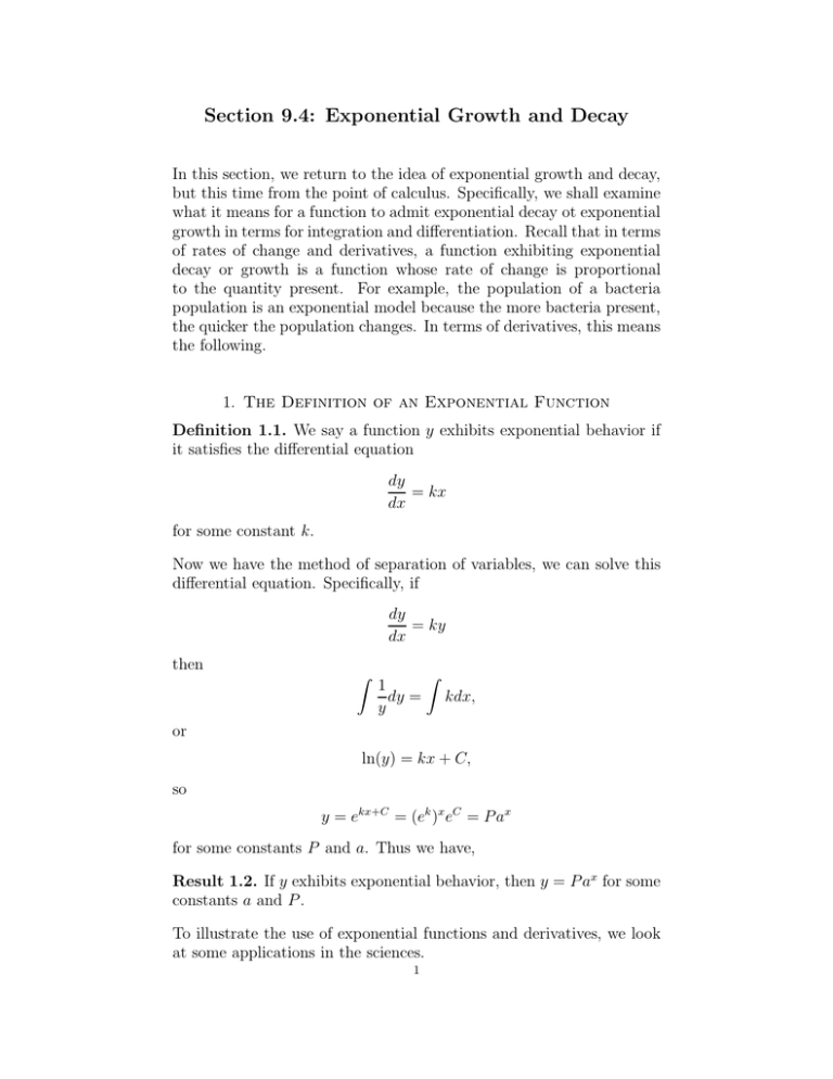
Section 9.4: Exponential Growth and Decay
In this section, we return to the idea of exponential growth and decay,
but this time from the point of calculus. Specifically, we shall examine
what it means for a function to admit exponential decay ot exponential
growth in terms for integration and differentiation. Recall that in terms
of rates of change and derivatives, a function exhibiting exponential
decay or growth is a function whose rate of change is proportional
to the quantity present. For example, the population of a bacteria
population is an exponential model because the more bacteria present,
the quicker the population changes. In terms of derivatives, this means
the following.
1. The Definition of an Exponential Function
Definition 1.1. We say a function y exhibits exponential behavior if
it satisfies the differential equation
dy
= kx
dx
for some constant k.
Now we have the method of separation of variables, we can solve this
differential equation. Specifically, if
dy
= ky
dx
then
Z
1
dy =
y
Z
kdx,
or
ln(y) = kx + C,
so
y = ekx+C = (ek )x eC = P ax
for some constants P and a. Thus we have,
Result 1.2. If y exhibits exponential behavior, then y = P ax for some
constants a and P .
To illustrate the use of exponential functions and derivatives, we look
at some applications in the sciences.
1
2
2. Population Modeling (Social Sciences)
Clearly population models (with no additional outside influences like
food resources and space) exhibit exponential growth (have you ever
heard the expression ”there are more people alive today than have
ever been alive!”). For population growth, people talk about a concept
called the ”Relative Growth Rate” or ”Rate of Growth”.
Definition 2.1. Suppose a population is modeled by the exponential
model
dP
= kP.
dt
Then we call the constant k the relative growth rate, so
k=
1 dP
.
P dt
So for example, if the relative growth rate of a population is 3% then
the population P will satisfy the differential equation
dP
= 0.03P.
dt
We illustrate with an example.
Example 2.2. A bacteria culture starts with 500 bacteria and grows
at a rate proportional to its size. After 3 hours, there are 8000 bacteria.
(i ) Find an expression for the number of bacteria after t hours.
We know that P = P0 at for some constants P0 and a.
Since the initial population is 500, we must have P0 = 500.
To calculate a, we observe that P (3) = 500a3 = 8000, so
a3 = 4000/500 = 9 or a = 2. Thus a model for the bacteria
population will be P (t) = 500 · 2t .
(ii ) What is the growth rate?
To find the growth rate, we need to find the value k where
dP
= kP.
dt
Calculating, we have
dP
= ln(2)500 · 2t = ln(2)P,
dt
so the relative growth rate is ln (2).
3. Radioactive Decay (Nuclear Physics)
Examples for this are very traditional Calc 1 and precalc material, so
we will not rehash old stuff!
3
4. Newtons Law of Cooling (Physics)
Let T (t) be the temperature of an object at time t and TS be the
temperature of the surroundings. Then Newton’s law of cooling says
that T satisfies the differential equations
dT
= k(T − TS )
dt
where k is some constant. It can be used to calculate the temperature
of an object which is different from its surroundings at any given time
t. We illustrate with an example.
Example 4.1. A freshly brewed cup of tea has temperature 100 degrees centigrade in a room of temperature 20 degrees. When the temperature is 70 degrees, it is cooling at a rate of 1 degree per minute.
When does this occur?
Let t = 0 be the time when the tea is brewed. We know when T = 70,
= −1. We know that T satisfies the differential
the rate of change dT
dy
dT
equation dt = k(T − TS ) where TS = 20, the temperature of the
surroundings. When T = 70, we have dT
= −1 = k(70 − 20) = 50k, so
dt
1
.
k = − 50
We need to find the time at which this temperature is achieved, so
1
= − 50
(T − 20). Using
we need to solve the differential equation dT
dt
separation of variables, we get
Z
Z
1
1
t
ln(T − 20) =
dT = − dt = − + C,
T − 20
50
50
and when t = 0, T = 100, so we get C = ln(80) giving
T = 80e−t/50 + 20.
When T = 70, we get 70 = 80e−t/50 + 20, or
8
5
t = −50 ln( ) = 50 ln( ) ∼ 23.5 minutes.
8
5
5. Compounding of Interest (Business)
Banks compound interest to bank accounts in many different ways. In
general, if an amount A0 is invested at an interest rate r, compounded
n times per year, then the value of the account after t years is
nt
r
A(t) = A0 1 +
.
n
Alternatively, some banks considering compounding interest ”continuously” by allowing n → ∞ in the formula. Under this circumstance,
we get that the value after t years is
A(t) = A0 ert
4
and in particular, A satisfies the differential equation
dA
= rA.
dt
We look at an example.
Example 5.1.
(i ) If $3000 is invested at 5% interest, then find
the value of the investment at the end of 5 years if the interest is compounded a) annually, b) monthly, c) daily and d)
continuously. What pattern do you notice?
Using the formulas, we have
a) Annually:
5
.05
= 3828.84.
A(5) = 3000 1 +
1
b) Monthy:
5∗12
.05
A(5) = 3000 1 +
= 3850.08.
12
c) Daily:
5∗365
.05
= 3852.01.
A(5) = 3000 1 +
365
d) Continuously:
A(5) = 3000e(.05∗5 = 3852.08.
Observe that the more times we compound interest, the
closer the value comes to continuous compounding.
(ii ) If A(t) is the amount of the investment at time t, write a
differential equation and an initial condition for A(t).
A′ (t) = 0.05 ∗ (3000e0.05t ) = 0.05A(t).