Your Choice
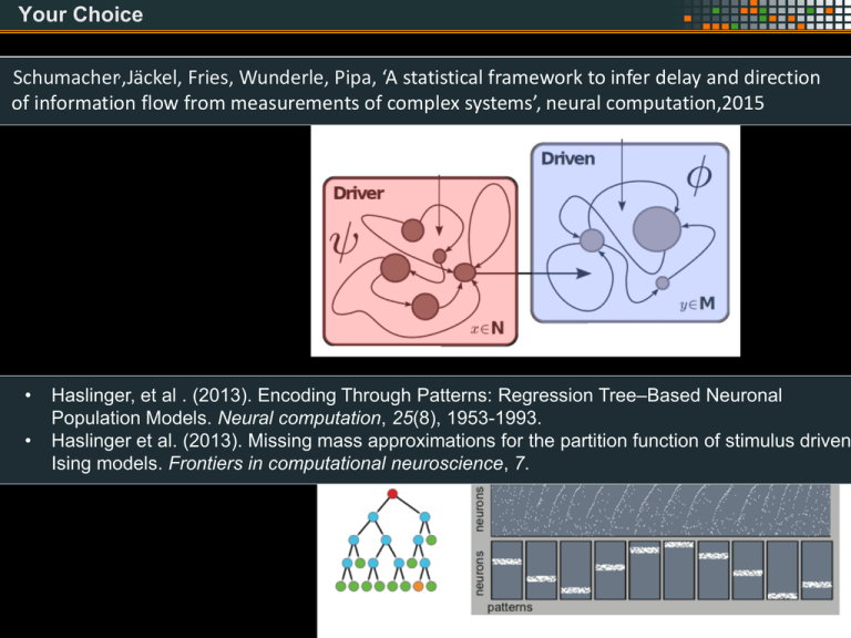
Schumacher,,Jäckel, Fries, Wunderle, Pipa, ‘A statistical framework
to infer
delay and direction
Johannes
Schumacher
of information flow from measurements of complex systems’, neural computation,2015
•
•
Haslinger, et al . (2013). Encoding Through Patterns: Regression
Tree–Based
Neuronal
Johannes
Schumacher
Population Models. Neural computation, 25(8), 1953-1993.
Haslinger et al. (2013). Missing mass approximations for the partition function of stimulus driven
Ising models. Frontiers in computational neuroscience, 7.
Gordon Pipa
Institute of Cognitive Science
Dept. Neuroinformatics
University of Osnabrück
Inferring functional interactions from neuronal
data
Johannes Schumacher1
Frank Jäckel1
Pascal Fries2
Thomas Wunderle2
1 Institute
2
of Cognitive Science - University of Osnabrück
Ernst Strüngmann Institute (ESI) , Frankfurt, Germany
The Brain: An ordered hierarchical system
Hagmann et al. (2008), ’Mapping the
structural core of human cerebral cortex’
PLoS Biol 6(7): e159
A dynamical system that is composed of coupled modules
Methods to detect causal Drive
Granger type
xt+1
xt,t:t
L(xt+1|xt,t:t , yt,t:t)
L(xt+1|xt,t:t)
yt,t:t
xt,t:t
L(yt+1|xt,t:t , yt,t:t)
L(yt+1| yt,t:t)
yt,t:t
L(xt+1|xt,t:t , yt,t:t)
L(xt+1|xt,t:t)
>
L(yt+1|xt,t:t , yt,t:t)
L(yt+1| yt,t:t)
YX
Methods to detect causal Drive
Many faces of Granger Causality:
• Spectral, auto-regressive, multivariate, state space, nonlinear, kernelbased, Transfer-Entropy, etc.
• Basically, G-Causality is a comparison of auto-prediction with a
cross-prediction
•
•
•
•
•
Granger, C. W. J. 1969 Investigating causal relations by econometric models and crossspectral methods. Econometrica 37, 424-438.
Granger, C. W. J. 1980 Testing for causality: A personal viewpoint. Journal of Economic
Dynamics and Control 2, 329-352.
Schreiber, T. 2000 Measuring information transfer. Phys Rev Lett 85, 461-4.
Vicente, Wibral, Lindner, Pipa, ‘Transfer entropy—a model-free measure of effective
connectivity for the neurosciences’, Journal of computational neuroscience 30 (1), 4567
……….
Methods to detect causal Drive
Using a dynamical system perspective
X
Y
Methods to detect causal Drive
Using a dynamical system perspective
X
X
Y
Y becomes a mix
of X and Y
Methods to detect causal Drive
Using a dynamical system perspective
X
X
Y
Y becomes a mix
of X and Y
Driven System:
System with m>n
dimensional
Driver System:
autonomous
System n dimensional
Schumacher, J., Wunderle, T., Fries, P., Jäkel, F., & Pipa, G. (2015). A Statistical Framework to Infer Delay
and Direction of Information Flow from Measurements of Complex Systems. Neural computation.
Methods to detect causal Drive
Using a dynamical system perspective
X
X
Y
Y becomes a mix
of X and Y
Reconstruction of past
X Y
X
X
X Y
Network topology: Common drive
Common driving with
unidirectional connections
1
3
2
Coupling Matrix
1→1
2→1
3→1
1→2
2→2
3→2
1→3
2→3
3→3
Color code:
coupled
uncoupled
Sugihara, G., May, R., Ye, H., Hsieh, C. H., Deyle, E., Fogarty, M., & Munch, S. (2012).
Detecting causality in complex ecosystems. science, 338(6106), 496-500.
Causality in a Dynamical System
Driven System:
System m>n
dimensional
Driver System:
autonomous
System n dimensional
Schumacher,,Jäckel, Fries, Wunderle, Pipa, ‘A statistical framework to infer delay and direction
of information flow from measurements of complex systems’, neural computation,2015
Formalizing the problem
Driven System:
System with m>n
dimensional
Driver System:
autonomous
System n dimensional
Stochastic or
partly observed
drive (highdimensional nonreconstructible
input)
Schumacher,,Jäckel, Fries, Wunderle, Pipa, ‘A statistical framework to infer delay and direction
of information flow from measurements of complex systems’, neural computation,2015
Formalizing the problem
Driven System:
System with m>n
dimensional
Driver System:
autonomous System
n dimen-sional
Stochastic or partly
observed drive
(high-dimensional
non-reconstructible
input)
Observable:
A set of scalar
observables
(e.g. LFP channels)
Schumacher,,Jäckel, Fries, Wunderle, Pipa, ‘A statistical framework to infer delay and direction
of information flow from measurements of complex systems’, neural computation,2015
P-Observable:
That means we can go back and forth between Recd and initial condition x,
or we can reconstruct system dynamics from observation
•
•
•
Aeyels D (1981) Generic observability of differentiable systems. SIAM Journal on Control and
Optimization 19: 595{603}.
Takens F (1981) Dynamical systems and turbulence, warwick 1980: Detecting strange attractors in
turbulence. In: Lecture Notes in Mathematics, Springer, volume 898/1981. pp. 366{381}
Takens F (2002) The reconstruction theorem for endomorphisms. Bulletin of the Brazilian Mathematical
Society 33: 231{262.
Causality in a Dynamical System
Forced Takens Theorem by Stark:
Stark J (1999) Delay embedding's for forced systems.
i.e deterministic forcing. Journal of Nonlinear
Science 9: 255{332.
That means we can can reconstruct the
driver x from the driven system y
Reconstruction in the presence of noise
Bundel embedding for noisy measurements:
(Stark J, Broomhead DS, Davies M, Huke J (2003) Delay
embeddings for forced systems. i.e. stochastic forcing.
Journal of Nonlinear Science 13: 519{577.)
That means we can define an
embedding for noisy measurements of
the driven systems, and reconstruct the
driver
Causality in a Dynamical System
P-Observable:
Driven system
To reconstruct
the driver we
reconstruct F,
that is the
projected skew
product on the
manifold N and
used the
measurement
function g
Causality in a Dynamical System
Driver
Driven
Causality in a Dynamical System
Driver
Driven
Causality in a Dynamical System
Driver
Driven
Moreover F is parameterized by a Volterra Kernel, leading
to a Gaussian Process Framework
Statistical Model
• Use of finite Order Volterra models with L1 (~ Identification of best
embedding )
• Alternatively we use infinite Order Volterra Kernel in Hilbert space (no
explicit generative model anymore)
• Model of posterior of predicted driver – Predictive distribution
• Extremely few data points are needed compared to information
theoretic approaches
Summary I
• If system A drives B the information of A and B is in B
• Than, one can reconstruct A from B using an embedding, but
not B from A
• This works if both system are represented by noisy measure,
this includes both real noise and incomplete observations
• To reconstruct A we model F based on a Volterra Kernel and
Gaussian process assumption
Delay-coupled Lorenz-Rössler System
Grating, cat, A18 and A21, 50 trials, rec. dimension d = 20, Recd spans an area
of 300ms
• Only one model for every direction. Compared to Granger
where we do not have to compare the auto with cross model
which prevents false detection because of bad auto models.
• Works for weak and intermediate coupling strength
• Formulates a non-linear statistical model, therefore enables
the use of state of the art machine learning
• Uses a Bayesian model which enables the use of predictive
distributions therefore allowing for a simple and fully intuitive
model comparison
Gordon Pipa
Institute of Cognitive Science
Dept. Neuroinformatics
University of Osnabrück
Inferring functional interactions from neuronal
data
Robert Haslinger3,4
Laura Lewis3
Danko Nikolić2
Ziv Williams4
Emery Brown3,4
1 Institute
of Cognitive Science - University of Osnabrück
and Cognitive Sciences, MIT, Cambridge, US
4 Massachusetts General Hospital , Boston, US
3 Brain
Assembly coding and temporal coordination
Hypothesis: Assembly coding and temporal coordination
Temporally coordinated activity of groups of neurons (assemblies) processes and stores
information, based on coordination emerging from interactions in the complex neuronal network.
• Hebb, ‘Organisation of behaviour. A neurophysiological theory’ , New York: John Wiley & Sons, 1949
• Uhlhaas, Pipa, Lima, Melloni, Neuenschwander, Nikolić, Singer, ‘Neural synchrony in cortical networks: history, concept
and current status’, Frontiers in integrative Neuroscience, 2009
• Vicente, Mirasso, Fischer, Pipa, ‘Dynamical relaying can yield zero time lag neuronal synchrony despite long conduction
delays, PNAS 2008
• Pipa , Wheeler , Singer , Nikolić, ‘NeuroXidence: reliable and efficient analysis of an excess or deficiency of joint-spike
events’, J. comp. neuroscience 2008
• Pipa, Munk, ‘Higher order spike synchrony in prefrontal cortex during visual memory ‘, Frontiers in Comp. neuros-, 2011
Data:
Task:
NeuroXidence:
2 simultaneously recorded cells, 38 trials
Delayed pointing
Number of surrogates: S = 20
Monkey primary motor cortex (awake)
Riehle, et al. 97 Science
Window length: l=0.2 s
PS
ES1
ES2
ES3
RS
G Pipa, A Riehle, S Grün, ‘Validation of task-related excess of spike coincidences based on NeuroXidence’, Neurocomputing
70 (10), 2064-2068
Synchrony should vary in time to be computationally relevant
Data:
Task:
NeuroXidence:
2 simultaneously recorded cells, 38 trials
Delayed pointing
Number of surrogates: S = 20
Monkey primary motor cortex (awake)
Riehle, et al. 97 Science
Window length: l=0.2 s
PS
ES1
ES2
ES3
RS
G Pipa, A Riehle, S Grün, ‘Validation of task-related excess of spike coincidences based on NeuroXidence’, Neurocomputing
70 (10), 2064-2068
Performance related cell-assembly formation
Dataset:
Monkey prefrontal cortex
Short term memory, delayed
matching to sample paradigm
27 cells simultaneously
recorded cells
Number of
different
Patterns :
18150
Pipa, G., & Munk, M. H. (2011). Higher order spike synchrony in prefrontal cortex during visual
memory. Frontiers in computational neuroscience, 5.
Challenges to overcome
• We are interested in how patterns encode that is how their probabilities vary with a
multidimensional external covariate (a stimulus).
• So the grouping should reflect the encoding ... but we don’t know how the groups.
• We have no training set telling us the probabilities, we have multinomial observations from
which we have to infer the probabilities.
• We also don’t know the functional form these probabilities should take, that is, the mapping
from stimulus to pattern.
• We will use a divisive clustering algorithm (hopefully ending up with the right clusters)
• This clustering will be constructed to maximize the data likelihood, and hopefully
generalize to test data.
• We will use an iterative expectation maximization type splitting algorithm.
•
•
Haslinger, R., Pipa, G., Lewis, L. D., Nikolić, D., Williams, Z., & Brown, E. (2013). Encoding Through Patterns:
Regression Tree–Based Neuronal Population Models. Neural computation, 25(8), 1953-1993.
Haslinger, R., Ba, D., Galuske, R., Williams, Z., & Pipa, G. (2013). Missing mass approximations for the partition
function of stimulus driven Ising models. Frontiers in computational neuroscience, 7.
Temporally Bin
Patterns
M unique patterns
neurons
1
Split into C clusters
M
Identify Patterns
Cluster Patterns
(But how ?)
Encoding with Patterns:
Patterns with the same temporal profile of p(t) belong to the same assemblies
•
•
Haslinger, R., Pipa, G., Lewis, L. D., Nikolić, D., Williams, Z., & Brown, E. (2013). Encoding Through Patterns:
Regression Tree–Based Neuronal Population Models. Neural computation, 25(8), 1953-1993.
Haslinger, R., Ba, D., Galuske, R., Williams, Z., & Pipa, G. (2013). Missing mass approximations for the partition
function of stimulus driven Ising models. Frontiers in computational neuroscience, 7.
Discrete Time Patterns
Temporally Bin
Patterns
M unique patterns
m Î1¼M
Multiplicative Model
Pm
Pt (m | st ) = P(m)r(st )
mean pattern
probability
P(m) =
Tm
T
stimulus
modulation
stimulus
Lots of methods for estimating this
Use tree to estimate this.
Expectation Maximization Splitting Algorithm
logistic regression model
e± X (stim) b
P± =
1+ e± X (stim) b
X(s)b
M
log L = å log Lm
m=1
This algorithm maximizes the data likelihood. It does not
depend on patterns “looking similar” or some other prior,
although priors can be reintroduced
Generalizing to Novel Patterns
Test data may (will) have pattern not seen in training data
P(m | st ) = P(m)r(m | st )
Assign new patterns to leaf to
containing patterns which
which it is “closest” (has
smallest Hamming distance)
Generalizing to Novel Patterns
Test data may (will) have pattern not seen in training data
P(m | st ) = P(m)r(m | st )
Problem:
Assigns zero
probability to
all patterns not
in training data
Good-Turing Estimator of
Missing Mass
P(m) =
Tm
T
a GT =
Number of patterns appearing once
Number of observations (T)
P(m) ® P(m)(1- a GT )
GT
P(m)
= a GT
P(m)ising
å
mÏdata
P(m)ising
2031 unique patterns,
many of which are very
rare
regression tree
recovered pattern groups
Independent neuron
group
The 10 correct pattern
groupings are recovered
Pattern Generation :
• multinomial logit model (One Pattern at a time)
• In total 60 neurons, for 100 sec
• Independent firing with 40 Hz for 92% of time
• 10 Groups that fire each at 0.8% of time.
• Each group composes 22 patterns
2031 unique patterns,
many of which are very
rare
regression tree
recovered pattern groups
Independent neuron
group
The 10 correct pattern
groupings are recovered
The covariation of the patterns probabilities with the stimulus is recovered
Cat V1 with grating stimulus
0.8 Hz Grating presented with
repeated trials
regression
tree in 12 directions
20 neuron population:
2600 unique patterns
parameterize stimulus as function of
patterns comprising 12 leaves
grating direction, and of time since
stimulus onset
V1 cat data from Danko Nikolic’
Compare regression tree to collection of independent neuron
models.
Bagged Training Data Log Likelihoods
E
1.6
1.2
1
0.8
10 -5
LL(null)
LL(stim)
1.4
original
shuffled
1.4
original
1.2
1
shuffled
0.8
10-4
10-3
10-2
10-1
100
101
0
regularization
0.02
0.04
missing mass
0.06
Bagged Test Data Log Likelihoods
1.05
original
0.95
0.9
0.85
-5
10
LL(null)
LL(stim)
1.4
1
shuffled
-4
10
original
1.2
1
shuffled
0.8
-3
10
-2
10
regularization
-1
10
0
10
1
10
0
0.02
0.04
missing mass
0.06
Compare regression tree to collection of independent neuron
models.
Good Turing Estimate
Ising model
Bagged Training Data Log Likelihoods
E
1.6
1.2
1
0.8
10 -5
LL(null)
LL(stim)
1.4
original
shuffled
1.4
original
1.2
1
shuffled
0.8
10-4
10-3
10-2
10-1
100
101
0
regularization
0.02
0.04
missing mass
0.06
Bagged Test Data Log Likelihoods
1.05
original
0.95
0.9
0.85
-5
10
LL(null)
LL(stim)
1.4
1
shuffled
-4
10
original
1.2
1
shuffled
0.8
-3
10
-2
10
regularization
-1
10
0
10
1
10
0
0.02
0.04
missing mass
0.06
One spike pattern
Two spike pattern
Three spike pattern
Temporal Profile
Pstim
1.5
1
0.5
0
1
sec. 2
3
2
3
2
3
Pstim
2
1
0
0
1
sec.
5
Pstim
Three Spike
Pattern
Two Spike
Pattern
One Spike
Pattern
Tuning Curves
0
0
1
sec.
Discussion and conclusion
Pattern encoding/decoding
• Grouping is based on just the temporal profile of pattern
occurrence
• Can work with very large numbers of neurons
• More Data  More detailed models
1
M
neurons
• Find the number of clusters automatically
• Generative model for encoding with patterns and independent
spiking
• Better than Ising Model
•
•
Haslinger, R., Pipa, G., Lewis, L. D., Nikolić, D., Williams, Z., & Brown, E. (2013). Encoding Through Patterns:
Regression Tree–Based Neuronal Population Models. Neural computation, 25(8), 1953-1993.
Haslinger, R., Ba, D., Galuske, R., Williams, Z., & Pipa, G. (2013). Missing mass approximations for the partition
function of stimulus driven Ising models. Frontiers in computational neuroscience, 7.
Encoding Based Pattern Clustering
Assume some patterns
convey similar information
about the stimulus
M unique patterns
M
neurons
1
Split into C clusters
e X (s ) b
P(m | s) =
1+ e X (s ) b
Use Regression Tree to
Divisively Cluster Patterns
Each split defined by a logistic regression
model dependent on stimulus
Leaves of tree are the pattern groupings
Tree is an stimulus encoding model for
each unique pattern observed
60 Simulated Neurons: 11 Functional Groups
1 independent neuron “group”
(Poisson firing)
Independent Firing
Collective Firing
10 “groups” of 6 neurons, each
with 22 unique patterns (4 or more
neurons firing)
a group is activated for certain
values of a time varying “stimulus”
“Stimulus” is 24 dimensional: sine waves
of varying frequency and phase offset
3 out of 24
“Stimulus”
time
Encodings based upon patterns can be compared to encodings
based upon independent neurons.
Do model comparison with log likelihood which is additive
Pt (m | st ) = P(m)r(m | st )
Comparing Tree Based and Independent Models
LL
tree indep
/LL
null
null
10
cell assemblies
randomized cell assemblies
8
6
4
2
0
0
1
2
3
4
5
6
7
8
9
10
11
9
10
11
% of time cell assemblies appear
Depends on
covariation of
pattern probability
with stimulus
LL
Depends on mean
probability (over all
stimuli) of observing
the pattern
indep
tree
/LL
stim
stim
6
5
4
3
2
1
0
0
1
2
3
4
5
6
7
8
% of time cell assemblies appear