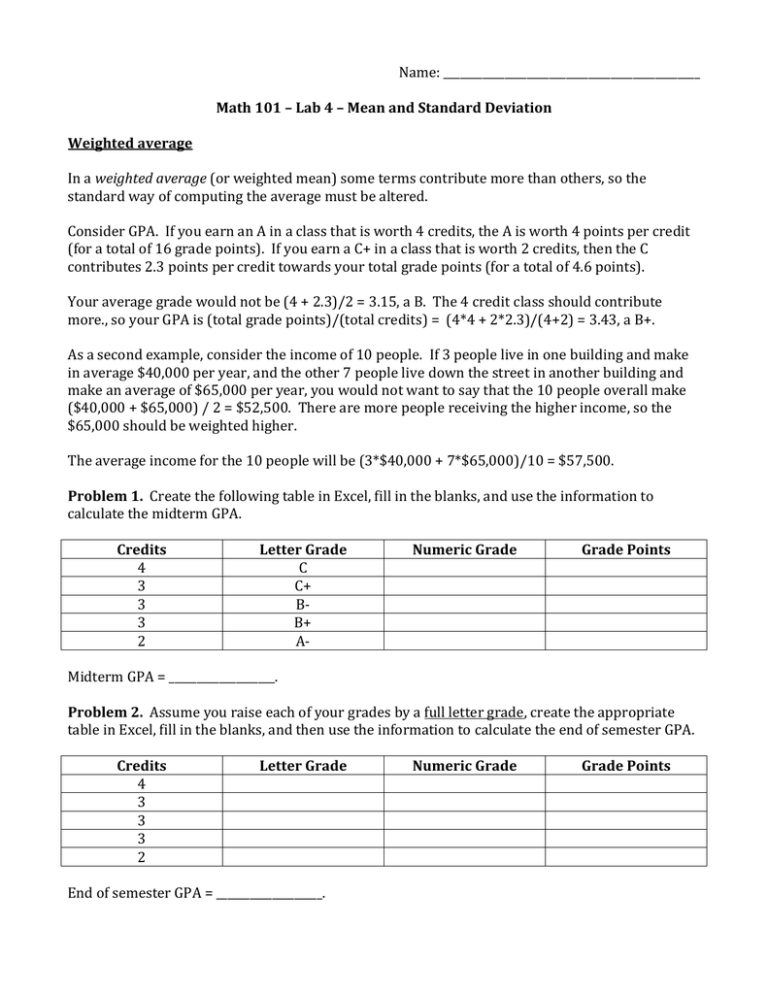
Name: ______________________________________________
Math 101 – Lab 4 – Mean and Standard Deviation
Weighted average
In a weighted average (or weighted mean) some terms contribute more than others, so the
standard way of computing the average must be altered.
Consider GPA. If you earn an A in a class that is worth 4 credits, the A is worth 4 points per credit
(for a total of 16 grade points). If you earn a C+ in a class that is worth 2 credits, then the C
contributes 2.3 points per credit towards your total grade points (for a total of 4.6 points).
Your average grade would not be (4 + 2.3)/2 = 3.15, a B. The 4 credit class should contribute
more., so your GPA is (total grade points)/(total credits) = (4*4 + 2*2.3)/(4+2) = 3.43, a B+.
As a second example, consider the income of 10 people. If 3 people live in one building and make
in average $40,000 per year, and the other 7 people live down the street in another building and
make an average of $65,000 per year, you would not want to say that the 10 people overall make
($40,000 + $65,000) / 2 = $52,500. There are more people receiving the higher income, so the
$65,000 should be weighted higher.
The average income for the 10 people will be (3*$40,000 + 7*$65,000)/10 = $57,500.
Problem 1. Create the following table in Excel, fill in the blanks, and use the information to
calculate the midterm GPA.
Credits
4
3
3
3
2
Letter Grade
C
C+
BB+
A-
Numeric Grade
Grade Points
Midterm GPA = ___________________.
Problem 2. Assume you raise each of your grades by a full letter grade, create the appropriate
table in Excel, fill in the blanks, and then use the information to calculate the end of semester GPA.
Credits
4
3
3
3
2
Letter Grade
End of semester GPA = ___________________.
Numeric Grade
Grade Points
Problem 3. Create the table below in Excel, fill in the blanks, and use it to determine the overall
GPA.
Semester
1
2
3
4
Total Credits
18
15
17
17
GPA
3.8
2.7
3.2
3.3
Total Grade Points
Cumulative GPA = ________________________.
Create a line chart showing the GPA over time.
Standard Deviation
Consider the following data about the number of sales per week at two different dealerships:
Weekly sales
4
5
6
7
8
9
10
Number of occurrences (frequency)
Dealership A
Dealership B
2
15
3
0
9
1
20
12
14
15
3
48
1
13
Problem 4. Enter the data for Dealership A and Dealership B into Excel (create 2 different tables,
Dealership A first and then Dealership B below it).
Next to the frequency for each dealership, use Excel to find the relative frequency (add this to you
table):
1
2
3
4
5
A
Dealership A
Weekly Sales
4
5
…
B
C
Frequency
2
3
…
Rel. Freq
??
??
…
Create a chart in Excel of the relative frequencies for each dealership.
Problem 5. For each dealership, find the mean number of weekly sales. Be careful, you have to
take a weighted mean (just like for the GPA calculations). For example, for Dealership A, 4 sales in
one week happens twice, 5 sales in one week happens 3 times, etc.
If you were buying a car dealership based on which one sells more cars per week on average,
which one would you pick?
Computing the standard deviation.
Recall that the distribution of a data set describes the values taken on and their frequencies. To
describe the distribution we have statistical variables such as range (max value – min value), mean
(average), median (middle point of values), and mode. It is also possible to discuss how the
distribution is skewed (left or right or not at all).
Variation describes how spread out the data is from the center. One way to measure and display
variation is with the 5-number summary and the accompanying box plot. The five numbers in the
5-number summary split the collection of values into quarters.
Another way to describe variation is with the standard deviation. It’s a measure of how far your
data points are from the mean. The larger the standard deviation, the more spread out.
Standard deviation =
sum of (data value  mean) 2
number data values 1
To compute this:
1.
2.
3.
4.
5.

Find the mean of your data set.
For each data point, take (data point – mean)2.
Add this up for every data point.
Divide by the number of data points -1.
Take the square root of this.
Problem 6. For the following data points, find the mean and compute the standard deviation:
1, 2, 3, 6, 7, 9
Here’s how to set it up in Excel:
A
B
1 Data Points
Points - mean
2
1
=(A2 – mean)
3
2
etc.
4
3
5
6
6
7
7
9
8 Compute the
mean here
C
Squared
=B2^2
etc.
D
E
Sum up the
squared terms
Take the square
root of the sum
divided by (6 – 1)
 this is the
standard
deviation
Problem 7. Do the same thing and find the standard deviation for the following data:
2, 3, 4, 4, 5, 5
Which of the two data sets is more spread out?
Note: There are built in functions in Excel to fid the mean and standard deviation: average() and
stdev(). Try using them and check that you get the same result as above.
Problem 8. Now using Excel, find the standard deviation for the weekly sales data for each
dealership.
You can use the following table to do this calculation:
1
A
B
Dealership A
2
Weekly
Sales
3
4
4
5
5
6
7
8
9
10
6
7
8
9
10
11
Freq
2
3
9
20
14
3
1
C
D
Sales x
Freq.
Data value
– mean
=A3*B3
=A3 – C12
E
F
Previous
column
squared
=(D3)^2
Multiply by
number of
data points
=E3 * B3
G

Total
number
of weeks
Sum (sales
x freq)
Sum up
above
Mean
=C10/B10
Standard
Deviation
12
13
=sqrt(F11/(B11-1))
Which dealership shows greater variation in their number of weekly sales? Which dealership is
more consistent in their sales?
Lab is due Monday, April 16th. Turn in your handout and email me your Excel
file: cthatcher@simons-rock.edu