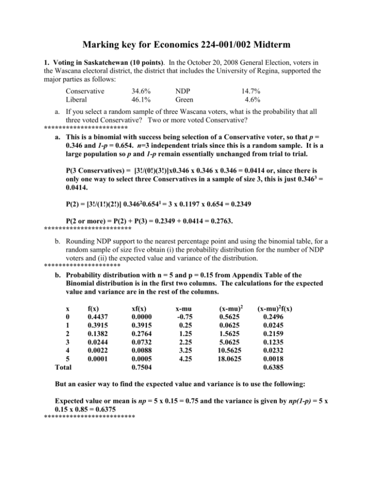
Marking key for Economics 224-001/002 Midterm
1. Voting in Saskatchewan (10 points). In the October 20, 2008 General Election, voters in
the Wascana electoral district, the district that includes the University of Regina, supported the
major parties as follows:
Conservative
Liberal
34.6%
46.1%
NDP
Green
14.7%
4.6%
a. If you select a random sample of three Wascana voters, what is the probability that all
three voted Conservative? Two or more voted Conservative?
***********************
a. This is a binomial with success being selection of a Conservative voter, so that p =
0.346 and 1-p = 0.654. n=3 independent trials since this is a random sample. It is a
large population so p and 1-p remain essentially unchanged from trial to trial.
P(3 Conservatives) = [3!/(0!)(3!)]x0.346 x 0.346 x 0.346 = 0.0414 or, since there is
only one way to select three Conservatives in a sample of size 3, this is just 0.3463 =
0.0414.
P(2) = [3!/(1!)(2!)] 0.34620.6541 = 3 x 0.1197 x 0.654 = 0.2349
P(2 or more) = P(2) + P(3) = 0.2349 + 0.0414 = 0.2763.
************************
b. Rounding NDP support to the nearest percentage point and using the binomial table, for a
random sample of size five obtain (i) the probability distribution for the number of NDP
voters and (ii) the expected value and variance of the distribution.
*********************
b. Probability distribution with n = 5 and p = 0.15 from Appendix Table of the
Binomial distribution is in the first two columns. The calculations for the expected
value and variance are in the rest of the columns.
x
0
1
2
3
4
5
Total
f(x)
0.4437
0.3915
0.1382
0.0244
0.0022
0.0001
xf(x)
0.0000
0.3915
0.2764
0.0732
0.0088
0.0005
0.7504
x-mu
-0.75
0.25
1.25
2.25
3.25
4.25
(x-mu)2
0.5625
0.0625
1.5625
5.0625
10.5625
18.0625
(x-mu)2f(x)
0.2496
0.0245
0.2159
0.1235
0.0232
0.0018
0.6385
But an easier way to find the expected value and variance is to use the following:
Expected value or mean is np = 5 x 0.15 = 0.75 and the variance is given by np(1-p) = 5 x
0.15 x 0.85 = 0.6375
*************************
2. The world economy (10 points). The world economy has been in great turmoil over the last
few months. Consider the following data:
Price, July 2008
Price, August 2008
Price, Oct.17, 2008
$147US
$112US
$72US
$1.36
$1.31
$1.12
$0.99US
$0.95US
$0.85US
Crude Oil
US $/barrel
Gasoline C$ per litre
Canadian Dollar
(US$ per C$)
a. Using the three data points on each variable as representative of the relationship between the
variables, draw two separate scatter graphs indicating your representation of the following:
 One showing the relationship between the price of crude oil and the price of gasoline.
 One showing the relationship between the price of crude oil and value of the
Canadian dollar.
Be sure to show more than just the 3 points on your estimated scatter graphs!
************************************************************************
The first graph below indicates the positive relationship between Crude Oil and gasoline
(A, B, C are July/Aug/Oct above), and the other graph the positive relationship between
crude oil and the C$. The x’s indicate some of the other points that must be present, but
which still show the positive relationship. (Graphs must be labelled).
P(Crude)
x
US$147
A
x
x
US$112
x
x
B
x
x
x
US$72
C
C$1.12
C$1.31
C$1.36 P(gas)
P(Crude)
x
US$147
A
x
x
US$112
x
x
B
x
x
x
US$72
C
0.85US$
0.95US$
0.99US$
US$ per C$
b. In addition, use this information to indicate what you think is the sign of the crosscorrelation coefficient between each pair of variables. Explain in a sentence or two why
you have picked that sign.
*********************
The sign in both cases is positive. As the Price of Crude Oil rises above the mean, so will
the price of gasoline (and ditto for the Canadian exchange rate), indicating a positive
relationship in the formula.
**********************
3. Student anti-poverty group (10 points). You and your friends are thinking about starting
an anti-poverty student group on campus. You would like to obtain information on the
percentage of students which would be supportive of such a group, and therefore you decide to
survey a set of U of R students. Two different approaches are suggested by your friends:
 Your friend Satish is in Business Administration. He argues that he should survey his
BUS 307 class, which has 80 students in it. He argues that given the size of his
survey, these will provide good results.
 Your friend Morgan is in English. Her favourite professor has agreed to let her
survey two different English 100 classes, with a total of 60 students in them. She
argues that since every student has to take English 100, she will have a sample that is
representative of the campus.
Explain what is good and what is flawed about each suggestion. Briefly provide and explain an
alternative sampling method that is more representative than these two.
*******************
Satish’s BUS 307 class has a fairly large class size. However, it will be principally Business
students, and unless we assume students with different majors have a similar set of
opinions, it will not be representative. It is also likely the students will be clustered in 3rd
year.
Morgan’s two classes will have a better range of majors, since all students must take
English 100 (although they may still be clustered, since some English sections are set aside
for individual majors). However, they are likely to be mostly first-year students, and so
once again are not representative.
Alternative methods might include
 Randomly interviewing students in a variety of buildings on campus at a variety of
times, and perhaps using weights to adjust for the information on majors that you could
get from the Office of Resource Planning webpage (OK, I don’t really expect you to
know the latter point).
 Ask for permission to email or mail all students.
**********************
4. Smoking behaviour and income (15 points). The data in Table 1 come from the
Saskatchewan respondents in Statistics Canada’s General Social Survey, Cycle 11, 1996.
Table 1. Number of adults cross-classified by number of cigarettes smoked daily and by household
income, Saskatchewan, 1996.
Number of
Cigarettes
Smoked Daily
Household Income
Less than
$30,000
$30,000 –
60,000
$60,000
plus
Total
209
369
128
706
1-10
17
32
12
61
11-20
44
74
11
129
Over 20
15
23
4
42
285
498
155
938
0
Total
a. Explain whether the following pairs of events are independent or dependent.
i. Smokes no cigarettes daily and is middle income ($30-60,000).
*********************
P(none) = 706/938 = 0.753
P(none/middle income) = 369/498 = 0.741
or
P(middle income) = 498/938 = 0.531
P(middle income/none) = 369/706 = 0.523
And since these two probabilities are very close to each other, the events of smoking no
cigarettes daily and being middle income are independent of each other.
******************************
ii. Smokes over 20 cigarettes daily and is from the highest income group.
**************************
P(over 20) = 42/938 = 0.045
P(over 20/highest income) = 4/155 = 0.0003
or
P(highest income) = 155/938 = 0.165
P(highest income/over 20) = 4/42 = 0.095
And since these two probabilities differ by a greater amount, the events of smoking over 20
cigarettes daily and being high income are dependent events.
****************************
b. “Lower income people are more likely to smoke.” Cite at least two probabilities that either
support or cast doubt on this statement and explain in a sentence or two.
****************************
There are many ways this could be analyzed. Here are three probabilities:
P(smoker/lowest income) = 1 – 209/285 = 1 – 0.733 = 0.267
P(smoker/middle income) = 1 – 369/498 = 1 – 0.741 = 0.259
P(smoker/high income) = 1 – 128/155 = 1 – 0.826 = 0.174
And as income goes from highest to lowest, the proportion of those who smoke at least
some each day increases. Note though that the large difference is between the highest
income group and those at lower to middle income. The middle and lower income groups
appear fairly similar in terms of their smoking behavior. As a result, it is not entirely clear
that the statement is correct – further analysis of smoking patterns by income would be
advisable.
*********************************
c. What is the 99% interval estimate for the proportion of Saskatchewan adults who smoke more
than 10 cigarettes daily? In a sentence or two, explain what the interval estimate means.
******************************
p is the unknown proportion of Saskatchewan adults who smoke more than 10 cigarettes
daily. The sample proportion is p = (129 + 42)/938 = 171/938 = 0.182. Since n = 938 is
large (n p = 938 x 0.182 = 171 and n(1- p ) is even larger) the distribution of p is
approximated by a normal distribution with mean p and standard deviation
p(1  p)
0.182  0.818
0.1448876


 0.0001587  0.0126
n
938
938
For 99% confidence, the appropriate Z value is 2.576 and the interval is
p ± (2.576 x 0.0126) = 0.182 ± 0.03246 or from 0.150 to 0.214, or (0.150, 0.214).
99% of samples yield intervals that contain the true proportion. The above interval may or
may not contain the true proportion of Saskatchewan adults who smoke more than 10
cigarettes daily but it probably does, since 99% of random samples yield intervals that
contain the population proportion.
***************
5. Immigration status and earnings (15 points). Historically, earnings of immigrants to
Canada have quickly matched or surpassed the earnings of the Canadian born. In recent years,
researchers have shown that immigrant earnings have fallen behind those born in Canada. To
investigate this, examine the data in Table 2, from a sample of Alberta adults in the Survey of
Income and Labour Dynamics (SLID).
Table 2. Means and standard deviations (in dollars) of earnings of Alberta adults by
immigrant/Canadian born status, 2004.
Statistic
Immigrant
Canadian born
Mean
38,100
41,200
Standard deviation
36,000
40,200
408
1,603
Sample size
a. Obtain the 95% interval estimate for the mean earnings of all Alberta immigrant workers
and all Alberta Canadian born workers.
*****************
Let μ be the mean income of all Alberta immigrant workers. Since n = 408 is large, the
normal distribution can be used to approximate the sampling distribution of the sample
mean. For 95% confidence, Z=1.96 and the intervals is
xZ

n
 x  1.96
36,000
36,000
 x  1.96
 x  3,493
20.199
408
This interval is from 38,100 – 3,500 = 34,600 to 38,100 + 3,500 = 41,600 or (34,600 , 41,600).
For this interval, the sample standard deviation of s = 36,000 has been used as an estimate
of the population standard deviation σ since the latter is unknown. This is generally
considered acceptable if the sample is a random sample and the sample size n is large.
For all the Canadian-born, the procedure is the same and the interval is
xZ

n
 x  1.96
40,200
40,200
 x  1.96
 x  1,968
40.037
1,603
or 41,200 – 2,000 = 39, 200 to 41,200 + 2,000 = 43,200.
Immigrant
Canadian-born
***************
Mean
95% interval
38,100
(34,600 , 41,600)
41,200
(39,200 , 43,200)
b. What is the sample size required in order to obtain an estimate of the mean income of all
immigrant workers in Alberta, correct to within $2,500, with probability 0.94?
*****************
For determination of sample size, assume that the sample size is large enough to have the
normal distribution approximate the distribution of the sample mean. For probability
0.94, there is 0.06 of the area in the two tails of the distribution, or 0.03 in each of the left
and right tails. The cumulative probability first reaches 0.03 at Z = -1.88 so this is the
appropriate Z. The estimate of the population standard deviation σ is s = 36 thousand (the
only indication available of what the variability of immigrant earnings is) and the required
margin of error is E = 2.5 thousand dollars. The required sample size is
 Z   1.88  36 
2
n
 
  27.072  732.9
 E   2.5 
2
2
And the required sample size is 733 immigrant workers. This assumes a random sample.
*****************
c. In a few sentences, explain whether the data in Table 2 and the interval estimates support
the argument that immigrants are falling behind Canadian born workers in terms of
earnings.
******************
The data in Table 2 support the contention in that the mean income of immigrant workers
is just over $3,000 lower than the income of the Canadian born in the sample.
Immigrant
Canadian-born
Mean
95% interval
38,100
(34,600 , 41,600)
41,200
(39,200 , 43,200)
However, the interval estimates have considerable overlap, meaning that the true mean for
all immigrant workers and all Canadian born workers could be similar, if data were to be
obtained from all of them, rather than just those in the sample.
There are other problems with this sample in that it does not distinguish age, sex,
occupation, experience, etc. for the two groups. A more detailed analysis of these
characteristics would be necessary to support the argument.
As a result, the data in Table 1 provides some support for the contention, but it is only
weak support.
***********************************
6. Canvassing for a non-profit organization (15 points). A nonprofit organization
conducting research on reducing cancer and improving the lives of cancer patients has hired you,
to explore ways of fundraising. You propose using volunteers to go door-to-door to canvass for
donations. You recruit volunteers to canvass seven city blocks in the area near the University
and the results of their canvass are given in Table 3.
Table 3. Donations obtained by seven canvassers
Canvasser
Donations
in dollars
Canvasser
Donation in
dollars
Kyle
70
Andrew
145
Samantha
30
Chen
75
Jing
123
Estelle
55
Rebecca
5
a. Calculate the mean, median, variance, and standard deviation of donations per city block.
**********************
xx
( x  x )2
70
-1.86
3.45
30
-41.86
1,752.02
123
51.14
2,615.59
5
-66.86
4,469.88
145
73.14
5,349.88
75
3.14
9.88
55
-16.86
284.16
503
14,484.86
The sum of the donations is $503 so the mean donation is 503/7 = $71.86.
The donations, in order from smallest to largest, are 5, 30, 55, 70, 75, 123, 145 and the
middle value is the 4th, or $70 is the median.
The sum of the squares of the differences from the mean is 14,484.86 and this divided by n
– 1 = 7 – 1 = 6 is 2,414.14 and this is the variance. The standard deviation is the square
root of this and is $49.13.
************************
b. Obtain the 98% confidence interval for an estimate of the mean amount of donations per
block for Regina, if all city blocks are canvassed. State any assumptions you adopt in
obtaining this estimate.
****************************
The sample size n = 7 is small and the standard deviation of the population σ is unknown,
so the sample mean has a t-distribution with n – 1 = 6 degrees of freedom and the standard
deviation is the sample standard deviation divided by the square root of 7. At 98%
confidence level, with 6 degrees of freedom, the t value is 3.143. This assumes that the
sample is a random sample from the population of all Regina city blocks.
x t
s
49.13
49.13
 x  3.143
 x  3.143
 x  58.36
2.646
n
7
The mean is $71.86 so the 98% interval estimate is 71.86 – 58.36 = 13.50 to 71.86 + 58.36 =
130.22 or ($13.50 , $130.22).
c. There are 2230 city blocks in Regina. What is the total amount of money you predict will
be raised? How accurate is this estimate likely to be? Recommend an improved
sampling procedure.
*************************
Using the sample mean to predict total donations for all of Regina, total donations would
be 2,230 x $71.86 = $160,247.80. However, this estimate is unlikely to be very accurate for
several reasons. The sample size is small, so the 98% interval is very wide. If the mean
amount raised per city block is at the low end of the interval, the total donations would
only be $30,105 although at the upper end they would be $290,390.60. This is such a large
difference, that one cannot be very sure what the donations would be.
In addition, the sample is not a random sample but is selected entirely from an area around
the University. These city blocks are unlikely representative of the whole city in terms of
donations, so an attempt should be made to obtain a more random or representative
sample of city blocks before making a prediction of total donations.
***************************