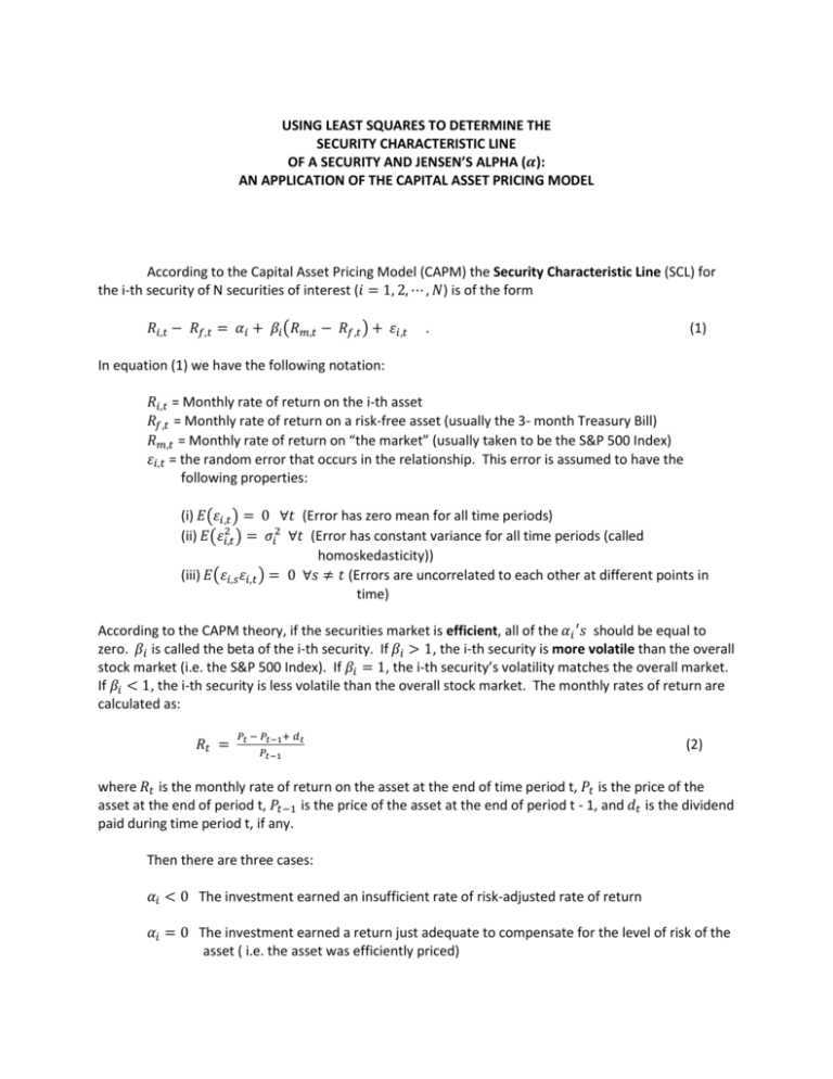
USING LEAST SQUARES TO DETERMINE THE
SECURITY CHARACTERISTIC LINE
OF A SECURITY AND JENSEN’S ALPHA ( ):
AN APPLICATION OF THE CAPITAL ASSET PRICING MODEL
According to the Capital Asset Pricing Model (CAPM) the Security Characteristic Line (SCL) for
the i-th security of N securities of interest (
) is of the form
(
)
.
(1)
In equation (1) we have the following notation:
= Monthly rate of return on the i-th asset
= Monthly rate of return on a risk-free asset (usually the 3- month Treasury Bill)
= Monthly rate of return on “the market” (usually taken to be the S&P 500 Index)
= the random error that occurs in the relationship. This error is assumed to have the
following properties:
(i) (
(ii) (
(iii) (
)
)
)
(Error has zero mean for all time periods)
(Error has constant variance for all time periods (called
homoskedasticity))
(Errors are uncorrelated to each other at different points in
time)
According to the CAPM theory, if the securities market is efficient, all of the
should be equal to
zero.
is called the beta of the i-th security. If
, the i-th security is more volatile than the overall
stock market (i.e. the S&P 500 Index). If
, the i-th security’s volatility matches the overall market.
If
, the i-th security is less volatile than the overall stock market. The monthly rates of return are
calculated as:
(2)
where is the monthly rate of return on the asset at the end of time period t, is the price of the
asset at the end of period t,
is the price of the asset at the end of period t - 1, and is the dividend
paid during time period t, if any.
Then there are three cases:
The investment earned an insufficient rate of risk-adjusted rate of return
The investment earned a return just adequate to compensate for the level of risk of the
asset ( i.e. the asset was efficiently priced)
The investment earned a superior risk-adjusted rate of return
Of course, the Jensen’s and the of the stock (or portfolio) are population parameters and must be
estimated. Least squares is traditionally used to estimate these parameters and their standard errors so
one can judge their significance.
Using the capm2.wf1 EVIEWS program and choosing the returns to General Motors stock to
analyze we can get a scatter plot of the data:
.3
.2
.1
Y
.0
-.1
-.2
-.3
-.20
-.15
-.10
-.05
.00
.05
X
Also we can apply least squares and get the following result:
Dependent Variable: Y
Method: Least Squares
Date: 01/20/11 Time: 13:17
Sample: 1 120
Included observations: 120
Variable
Coefficient
Std. Error
t-Statistic
Prob.
C
X
-0.002314
1.074415
0.007301
0.155765
-0.316978
6.897679
0.7518
0.0000
R-squared
Adjusted R-squared
S.E. of regression
Sum squared resid
Log likelihood
F-statistic
Prob(F-statistic)
0.287345
0.281305
0.078996
0.736361
135.3390
47.57798
0.000000
Mean dependent var
S.D. dependent var
Akaike info criterion
Schwarz criterion
Hannan-Quinn criter.
Durbin-Watson stat
0.005555
0.093182
-2.222317
-2.175859
-2.203450
2.226312
.10
The estimated Security Characteristic Line for General Motors stock can then be written in conventional
form as
̂
(0.007301) (0.155765)
Jenson’s estimated alpha is -0.002314 which is not statistically different from zero since its t-statistic is
-0.002314/0.007301 = -0.316978 with a two-sided probability value of p = 0.7518. Thus we can
conclude that during the period of the observed returns, that GM stock was efficiently priced (i.e. its
return is commensurate with the risk the stock carries). Also we can see that the beta of the GM stock is
not significantly different from 1 as the t-statistic for testing
versus
is t = (1.074415
– 1)/0.155765 = 0.074415/0.155765 = 0.4777 which has a two-sided probability value of p = 0.633747
which is statistically insignificant and thus we conclude that GM is not an overly aggressive stock or
overly conservative stock.