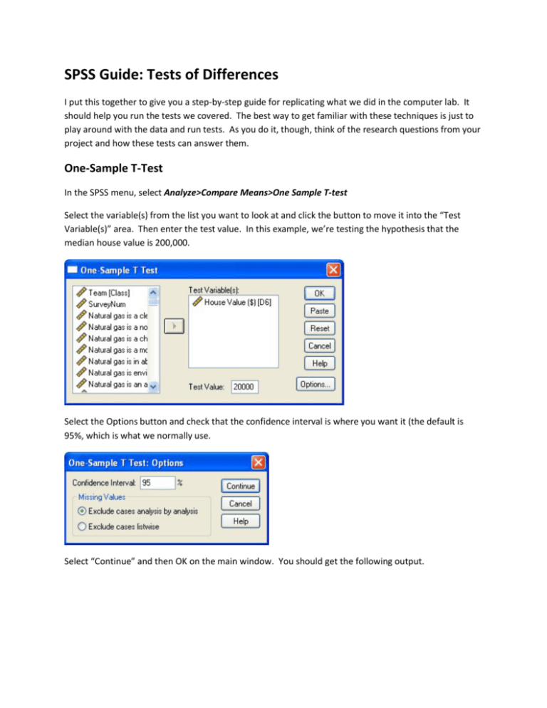
SPSS Guide: Tests of Differences
I put this together to give you a step-by-step guide for replicating what we did in the computer lab. It
should help you run the tests we covered. The best way to get familiar with these techniques is just to
play around with the data and run tests. As you do it, though, think of the research questions from your
project and how these tests can answer them.
One-Sample T-Test
In the SPSS menu, select Analyze>Compare Means>One Sample T-test
Select the variable(s) from the list you want to look at and click the button to move it into the “Test
Variable(s)” area. Then enter the test value. In this example, we’re testing the hypothesis that the
median house value is 200,000.
Select the Options button and check that the confidence interval is where you want it (the default is
95%, which is what we normally use.
Select “Continue” and then OK on the main window. You should get the following output.
One-Sample Statistics
N
D6 House Value ($)
Mean
1123
203786.40
Std. Deviation
Std. Error Mean
184926.607
5518.354
One-Sample Test
Test Value = 200000
95% Confidence Interval of the
Difference
t
D6 House Value ($)
df
.686
Sig. (2-tailed)
1122
.493
Mean Difference
3786.401
Lower
-7041.05
Upper
14613.85
Note that the mean is $203,786.40, which is pretty close to the hypothesized value. The significance is
.493, well above the .05 threshold, so our hypothesis is supported.
How do you know whether the significance should be higher or lower than .05? Recall that this is a test
of whether there is a statistical difference between the test value and the sample mean. Since the tvalue is not significant, we reject the null hypothesis that there is a difference, and accept our
hypothesis.
Independent Samples T-test
This test is similar to the one-sample test, except rather than testing a hypothesized mean, we’re testing
to see if there is a difference between two groups.
For the grouping variable, you can choose a demographic trait (such as gender, age, ethnicity, etc) or
any other variable that classifies your groups. (In an experimental design, it is a good way to test the
differences between the control group and the manipulation group.) In this example, we’ll use gender.
In the SPSS menu, select Analyze>Compare Means>Independent Samples T-test
Select your Test variable from the list. This is the variable for which you want to compare means. In this
example, we will test C18 (“I would describe myself as environmentally responsible.”)
Now select the grouping variable, which is the trait you’re using to divide the groups. For this example,
we will select gender. Select it from the list and click the arrow next to “Grouping Variable.”
Then, click “Define Groups …” and enter the values for the two groups. In this example, 1=Female and
2=Male. Also notice the “Cut Point” option. What if we wanted to divide the sample into two groups
based on home value? The cut point would be the value where you split the sample. For example, if
you entered 100,000, it would create two groups – one for home value less than 100,000 and another
for more than 200,000. For this example, let’s stick to gender, though. Select continue, and then click
“OK.” You’ll go back to the previous window with the groups fiilled in.
Select “OK”, and you’ll get the output on the following page. You’ll notice that the means appear to be
pretty close and the standard deviations are pretty close, too. So the means and distribution don’t
appear to be different, but we need to test it statistically. This one is similar to the one-sample test,
except first we have to test for equal variance.
Step One: Is there a difference in variance? If the Laverne’s Test is <.05, we assume unequal variances
and go to the second line. Otherwise, variances are equal, so we use the top test.
Step Two: Is there a difference in means? If the significance of the t-test is <.05, there is a difference in
means. If it is >.05, then the null hypothesis (no difference) is supported.
Group Statistics
D1 Gender
N
C18 I would describe myself 1 Male
as environmentally
2 Female
responsible
Mean
Std. Deviation
Std. Error Mean
886
3.32
.963
.032
782
3.38
.957
.034
Independent Samples Test
Levene's Test
for Equality of
Variances
t-test for Equality of Means
95% Confidence
Interval of the
F
C18 I would describe
Equal
myself as
variances
environmentally
assumed
responsible
.021
Sig.
t
df
Sig. (2-
Mean
Std. Error
tailed)
Difference
Difference
Difference
Lower
Upper
.886 -1.248
1666
.212
-.059
.047
-.151
.034
-1.249
1642.573
.212
-.059
.047
-.151
.034
Equal
variances not
assumed
The Laverne’s test of .886 indicates that we should assume equal variances.
The t-test significance is .212, so there does not appear to be a difference in means. The null hypothesis
is supported.
Paired Samples t-test
With the paired samples t-test, we’re not testing for differences between groups. Instead, we’re testing
for means of different variables within the sample sample.
For example, we want to compare the mean for user-created videos and the mean for companygenerated videos.
Go to Analyze>Compare Means>Paired Samples T-test
Select the two variables you want to compare, and click the arrow to move them into the “Paired
Variables” pane.
Under options, make sure that you’re using a 95% confidence interval.
Click continue and then OK and you’ll get the following output.
Paired Samples Statistics
Mean
Pair 1
N
Std. Error
Mean
Std. Deviation
C4 I like YouTube
videos created by the
sponsor company of
the product or brand
2.90
1274
1.191
.033
C5 I like YouTube
videos created by
customers/fans of the
product or brand
3.05
1274
1.183
.033
Paired Samples Correlations
N
Pair 1
C4 I like YouTube videos
created by the sponsor
company of the product or
brand & C5 I like YouTube
videos created by
customers/fans of the
product or brand
Correlation
1274
Sig.
.689
.000
Paired Samples Test
Mean
Pair
1
C4 I like YouTube
videos created by
the sponsor
company of the
product or brand C5 I like YouTube
videos created by
customers/fans of
the product or brand
-.146
Paired Differences
95% Confidence
Interval of the
Difference
Std.
Std.
Error
Deviation
Mean
Upper
Lower
.936
.026
-.197
-.095
Sig. (2tailed)
Std.
Err
or
Me
Std. Deviation
an
df
t
-5.568
1273
.000
Remember that the null hypothesis is that there is no difference between the means. Note that the
absolute value of the t-value is greater than the critical value (1.96). Since the significance is .000, which
is less than .05 we can reject the null hypothesis and conclude that there is a difference between the
two means. If you look at the descriptive statistics for the paired sample, you can see which mean is
greater.
One-Way ANOVA
What if we want to test for differences between more than two groups. ANOVA (which stands for
“Analysis of Variance”) is the way to go.
Analysis>Compare Means>One-Way ANOVA
Select the variable(s) you want to test and move into the “Dependent List” pane.
Now, move the variable that you are using to separate them into groups into the “Factor” pane. For
example, in our data set, there are three age groups (“1”,”2” and “3”) for the 15-18, 19-24, and 25+
groups, respectively, in the AgeGroup variable.
Click “OK” and you get the following output.
ANOVA
CON1
Sum of Squares
Between Groups
df
Mean Square
2.707
2
1.353
Within Groups
1081.801
1282
.844
Total
1084.508
1284
F
1.604
Sig.
.202
The F-test is less than the critical F-value (1.604<1.96). The significance of .202 is greater than .05, so we
fail to reject the null. There are no significant differences in the mean for CON1 between the three
groups. The test is complete.
But what if the test is significant?
ANOVA
CON2
Sum of Squares
Between Groups
df
Mean Square
21.145
2
10.572
Within Groups
931.955
1286
.725
Total
953.100
1288
F
14.589
Sig.
.000
The significance is .000, so we reject the null hypothesis and conclude that at least one of the means is
significantly different. But which one(s)? To determine this, we must use a post-hoc test. Go back to
Analyze>Compare Means>One Way ANOVA but this time, click Post-Hoc
Then, select “Tukey” and “Duncan”
You will get the following output for the Tukey test.
Post Hoc Tests
Multiple Comparisons
Dependent Variable:CON2
95% Confidence Interval
Tukey
(I) AgeGroup
(J) AgeGroup
AgeGroup
AgeGroup
1 15-18 year olds
2 19-24 year olds
.00831
.05820 .989
-.1282
.1449
3 25 years old +
.27527
*
.05816 .000
.1388
.4117
1 15-18 year olds
-.00831
.05820 .989
-.1449
.1282
3 25 years old +
.26696
*
.05789 .000
.1311
.4028
1 15-18 year olds
-.27527
*
.05816 .000
-.4117
-.1388
2 19-24 year olds
-.26696
*
.05789 .000
-.4028
-.1311
HSD
2 19-24 year olds
3 25 years old +
*. The mean difference is significant at the 0.05 level.
Mean Difference (I-
Std.
J)
Error
Sig.
Lower
Upper
Bound
Bound
Notice that the output compares the group in the left column with the other two groups in the right
column and gives you the significance level and the difference in means. The 25 year old + group is
significantly different (p=.000) than the other two groups, but there is no significant difference between
the 15-18 year olds and 19-24 year olds. The” mean difference” column indicates that I-J = .27527); that
is, the mean for 15-18 year-olds – mean for 25yo + = .27527. In other words, the mean for 15-18 year
olds is .27527 higher (on a 1-5 scale) than the 25+ yo.
Also, the Duncan and Tukey tests both create homogenous groups (“segments”, in strategy terms) based
on their means.
CON2
Subset for alpha = 0.05
AgeGroup
AgeGroup
a
Tukey HSD
N
1
3 25 years old +
433
2 19-24 year olds
432
3.6079
1 15-18 year olds
424
3.6162
Sig.
Duncan
a
2
3.3409
1.000
.989
3 25 years old +
433
2 19-24 year olds
432
3.6079
1 15-18 year olds
424
3.6162
Sig.
3.3409
1.000
.886
Means for groups in homogeneous subsets are displayed.
a. Uses Harmonic Mean Sample Size = 429.629.
As you would expect from the previous test, the 25+ group forms one segment and the other two age
groups form a second segment. The values (3.3409, etc.) are the means for each group.