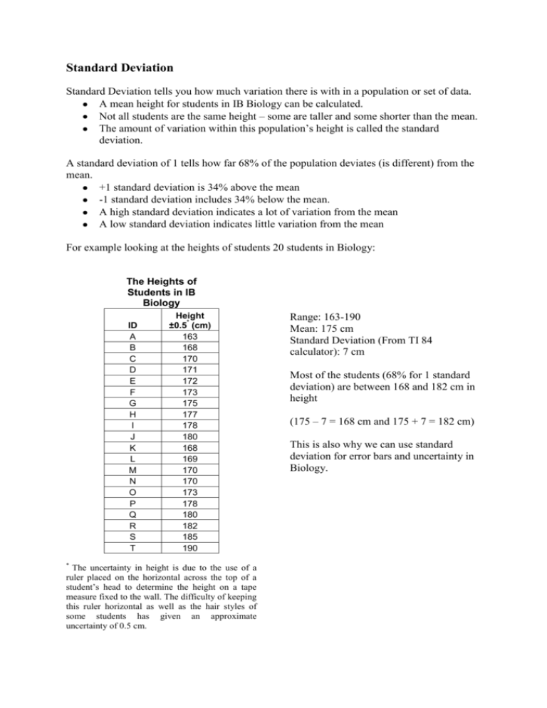
Standard Deviation
Standard Deviation tells you how much variation there is with in a population or set of data.
A mean height for students in IB Biology can be calculated.
Not all students are the same height – some are taller and some shorter than the mean.
The amount of variation within this population’s height is called the standard
deviation.
A standard deviation of 1 tells how far 68% of the population deviates (is different) from the
mean.
+1 standard deviation is 34% above the mean
-1 standard deviation includes 34% below the mean.
A high standard deviation indicates a lot of variation from the mean
A low standard deviation indicates little variation from the mean
For example looking at the heights of students 20 students in Biology:
The Heights of
Students in IB
Biology
ID
A
B
C
D
E
F
G
H
I
J
K
L
M
N
O
P
Q
R
S
T
*
Height
*
±0.5 (cm)
163
168
170
171
172
173
175
177
178
180
168
169
170
170
173
178
180
182
185
190
The uncertainty in height is due to the use of a
ruler placed on the horizontal across the top of a
student’s head to determine the height on a tape
measure fixed to the wall. The difficulty of keeping
this ruler horizontal as well as the hair styles of
some students has given an approximate
uncertainty of 0.5 cm.
Range: 163-190
Mean: 175 cm
Standard Deviation (From TI 84
calculator): 7 cm
Most of the students (68% for 1 standard
deviation) are between 168 and 182 cm in
height
(175 – 7 = 168 cm and 175 + 7 = 182 cm)
This is also why we can use standard
deviation for error bars and uncertainty in
Biology.
Standard deviation is also useful to see if the difference between the means of two sets of
data is significant or not. For example: Is there a significant difference between the heights of
girls and boys in IB Biology?
The Heights of Students in IB Biology
Female Students
Male Students
Height
Height
*
*
Student ID ±0.5 (cm) Student ID ±0.5 (cm)
A
163
K
168
B
168
L
169
C
170
M
170
D
171
N
170
E
172
O
173
F
173
P
178
G
175
Q
180
H
177
R
182
I
178
S
185
J
180
T
190
*
The uncertainty in height is due to the use of a ruler placed on the horizontal across the top of a student’s head
to determine the height on a tape measure fixed to the wall. The difficulty of keeping this ruler horizontal as
well as the hair styles of some students has given an approximate uncertainty of 0.5 cm.
Female studentsRange: 163-180 cm
Mean: 173 cm
Standard deviation: 5
(From TI 84 calculator):
Male StudentsRange: 168-190 cm
Mean: 177 cm
Standard Deviation: 8
(From TI 84 calculator):
Looking at the mean and standard deviation of each set, we can see that 68% of the female
population is between 168 and 178 cm in height while 68% of the male population is between
169 and 185 cm in height.
If the difference between the mean heights of male and female students was more than the
standard deviations of each, we could say there is a significant difference between the heights of
the two groups. But in our data above, there is an overlap between the heights of the tall girls and
the short boys even with in one standard deviation.
In this case we need to additionally use the T-Test to see if this overlap between the two groups
is significant or not.
Understanding the T-Test
The T-Test is a statistical test used to compare two sets of data to determine if there is a
significant difference between them.
The T-Test is based on the idea of a null hypothesis
A null hypothesis states “there is no difference between two sets of data.” The null hypothesis
may often be the opposite of your actual hypothesis.
Remember it is easier to disprove something rather than prove something. If you can prove your
null hypothesis to be wrong this means there IS a significant difference between the two sets of
data and this may give evidence to SUPPORT (not prove) your hypothesis.
IF there is a significant difference between your two sets of data THEN this may support your
claim that the difference is caused by your independent variable and not by random chance.
But, this claim may only be made as long as ALL other variables were completely controlled,
otherwise the difference may have been made by something else. Notice the T-Test can not tell
you if your hypothesis is supported, it ONLY tells you if there is a significant difference between
the two sets of data.
In using the data comparing the heights of female and male students in IB Biology we might
have a hypothesis stating that “If the height of students is mostly dependant on gender of the
students then there will be a significant difference between heights of the male and the female
students.”
The Null hypothesis would be: “there is no significant difference between the heights of the
male and female students.”
The T-Test will give us a probability of how true the null hypothesis is.
If there is a probability of greater than 0.05 (5%) than we must accept the possibility that the null
hypothesis is true and we would have to accept that any difference shown by the means of the
two populations is due to random chance. The experimental hypothesis above would then be
rejected (there is no significant difference between the heights of male and female students in IB
Biology).
If the probability is less than the 0.05 (5%) than we can reject the null hypothesis and state that
there is a significant difference between the heights of the two populations and that this may be
due to a variable other than random chance. In other words, as long as you have controlled all
variables carefully, this difference is likely caused by your independent variable – the gender of
the students.
Calculating the T-Test
You need two sets of data with at least 10 numbers in each set:
The Heights of Students in Grade 12 Biology
Female Students
Male Students
Height
Height
*
*
Student ID ±0.5 (cm) Student ID ±0.5 (cm)
A
163
K
168
B
168
L
169
C
170
M
170
D
171
N
170
E
172
O
173
F
173
P
178
G
175
Q
180
H
177
R
182
I
178
S
185
J
180
T
190
*
The uncertainty in height is due to the use of a ruler placed on the horizontal across the top of a student’s head to
determine the height on a tape measure fixed to the wall. The difficulty of keeping this ruler horizontal as well as the
hair styles of some students has given an approximate uncertainty of 0.5 cm.
Enter these as two lists into your TI Graphing Calculator or use Excel.
For the example above, on the TI 84:
1. Select “STAT” > “EDIT” > “1: Edit…”
2. Enter your two sets of data for comparison into separate lists
3. Select “STAT” > “TESTS” > “4: 2-SampTTest”
4. Check that the following are selected correctly:
Inpt: Data
List1: L1 (or the correct label of your first list)
List2: L2 (or the correct label of your second list)
Freq1: 1
Freq2: 1
μ1:≠ μ2
Pooled: Yes
5. Enter “Calculate”
From this data you should see:
t=-1.310… (This is the value for t. Ignore the negative sign)
p=.206… (This the probability that there is no difference in the data)
df=18 (degrees of freedom, you have a total of 20 values minus 2=18)
×1=172.7 (mean for list one)
×2=176.5 (mean for list two)
S×1=5.078… (standard deviation for list 1)
S×2=7.633… (standard deviation for list 1)
This will give you a number of statistics about your lists of data, including the mean of each, the
standard deviation of each and at the top, the value for T of each and the probability of the null
hypothesis being correct. Remember a probability of greater than 0.05 means there is not a
significant difference in your sets of data and your actual hypothesis may not be supported. A
probability of 0.05 or less means that the null hypothesis is rejected and you may accept your
actual hypothesis that there IS a significant difference between the two sets of data.
If you are comparing the value for T off of a table of critical values, you must also calculate the
degrees of freedom. To do this, you add together how many numbers you have in each set of data
and subtract by the number of sets. In this case we have 10 heights in each set and two sets;
therefore we have 18 degrees of freedom.
Find the number for T that corresponds to 18 degrees of freedom and a probability of 0.05. In
this case your number for T must be GREATER than or equal to this number. Notice that as the
probability decreases, the value for T increases.
To reject the null hypothesis that there is no difference and accept the experimental
hypothesis that there is a difference, T must be greater than 2.101 when you have 18
degrees of freedom.
Is the null hypothesis accepted or rejected for the data above?
Is your experimental hypothesis supported or rejected? Is there a significant difference between
the heights of female and male students in the IB Biology class?