Math 103, Summer 2006
Eigenvectors and Eigenvalues, Geometrically
August 1, 2006
EIGENVECTORS AND EIGENVALUES, GEOMETRICALLY
1. Announcements
There are things about the test people might be interested in. The first is that the material covered on this
coming midterm will focus mainly on material that we’ve covered since the first midterm (including the lecture
or two before the first midterm). Math exams are almost always cumulative in some way or another, but while
you will be required to know the topics we discussed in the first few weeks of class the test will ask questions
centered around the more recent material.
As for the first midterm, we’ll be holding a review session for this midterm. It will be held in room 380-C
(basement of the math building) and will start at 6pm. As last time I’ll bring pizza and drinks, and you should
bring lots of questions to ask.
2. Recap
Last class period we talked about how one goes about finding eigenvalues for a matrix A, and at the very
end of class we talked about a strategy for computing the corresponding eigenspaces. As a refresher, I’ll just
state the following
Definition 2.1. The eigenspace corresponding to an eigenvalue λ is the set
→
→
→
{−
v : A−
v = λ−
v }.
It is denoted Eλ .
We said in class yesterday that this is actually a subspace, and we asked the question: how does one compute
the eigenspace? More precisely, how can I find a basis for the eigenspace Eλ when I have an eigenvalue λ?
→
−
−
→
By the definition of Eλ we know that any −
v ∈ Eλ satisfies A→
v = λ→
v , which means that −
v ∈ ker(A − λIn ).
Hence to find Eλ , one just computes ker(A − λIn ).
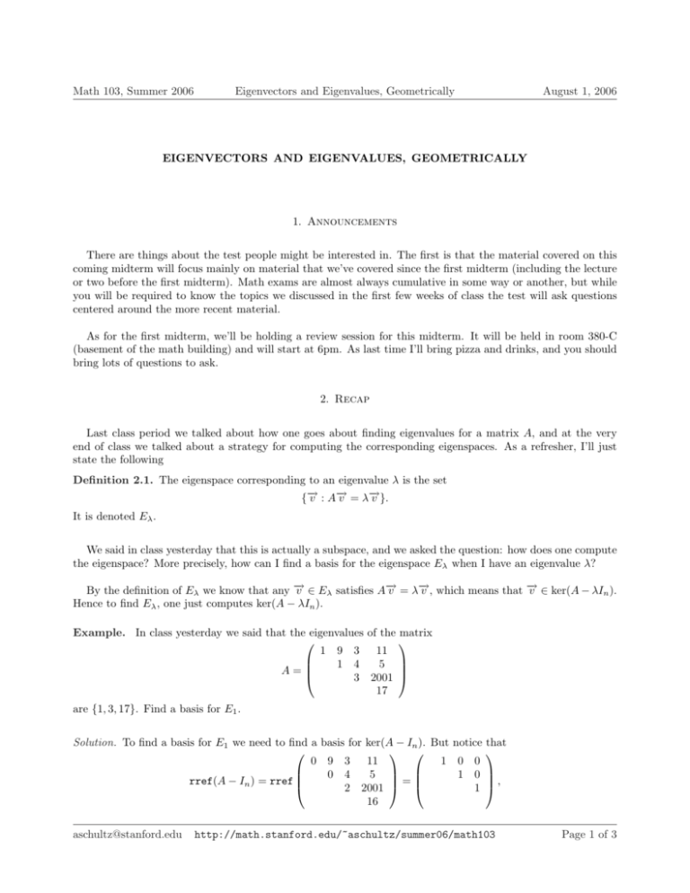
Example. In class yesterday we said that the eigenvalues of the matrix


1 9 3 11

1 4
5 

A=

3 2001 
17
are {1, 3, 17}. Find a basis for E1 .
Solution. To find a basis for E1 we need to find a basis for ker(A − In ). But notice

 
0 9 3 11
1 0 0

 
0
4
5
1 0
=
rref(A − In ) = rref 

2 2001  
1
16
aschultz@stanford.edu
that


,

http://math.stanford.edu/~aschultz/summer06/math103
Page 1 of 3
Math 103, Summer 2006
Eigenvectors and Eigenvalues, Geometrically
August 1, 2006



1
1
 0 
 0


and hence ker(A − In ) = Span(
 0 ). This means that E1 has a basis given by the vector  0
0
0


.

¤
Notice in this example that dim(E1 ) = 1, but that the algebraic multiplicity of λ = 1 was 2. The dimension
of an eigenspace captures important geometric information about the action of the matrix A, and hence has a
special name.
Definition 2.2. The geometric multiplicity of an eigenvalue λ is dim(Eλ ).
With this new language, our observation is that the geometric multiplicity of 1 was less than the algebraic
multiplicty of 1. In fact this is an example of a more general relationship.
Theorem 2.1. For an eigenvalue λ, the geometric multiplicty of λ is at most the algebraic multiplicty of λ.
Let’s do another example, but this time we’ll do the whole kit and kaboodle.
Example. Let
µ
A=
7
−3
−3
7
¶
.
→
Find all eigenvalues of A, a basis for all eigenspaces, and a formula for −
vt if
µ ¶
1
−
→
.
v0 =
2
Solution. To find the eigenvalues of A we must compute the roots of the characteristic polynomial
¶
µ
7−λ
−3
= (7 − λ)2 + 9 = ((7 − λ) − 3)((7 − λ) + 3) = (4 − λ)(10 − λ).
det(A − λI2 ) = det
−3
7−λ
Since we’ve factored the characteristic polynomial we can ‘see’ the eigenvalues are {4, 10}.
Now to find the corresponding eigenspaces, we find a basis for the kernels of appropriate matrices. For
instance, to find E4 I compute a basis for
¶
¶
µ
µ
¶
µ
3 −3
1 −1
7 − 4 −3
= ker
= ker
.
ker
0
0
−3
3
−3 7 − 4
But I can read off a basis of the kernel on the
µ right
¶ since my matrix is in reduced row echelon form, and I see
1
that E4 has a basis given by the the vector
.
1
Similarly, to find E10 I compute a basis for
µ
¶
µ
7 − 10
−3
−3
ker
= ker
−3
7 − 10
−3
−3
−3
¶
µ
= ker
1
0
1
0
¶
.
I can read µ
off a basis
¶ of the kernel on the right just like last time, and I see that E10 has a basis given by the
1
the vector
.
−1
aschultz@stanford.edu
http://math.stanford.edu/~aschultz/summer06/math103
Page 2 of 3
Math 103, Summer 2006
Eigenvectors and Eigenvalues, Geometrically
August 1, 2006
¶
1
→
−
. Now I know that −
v t = At →
v0 , but I also know this isn’t
2
−
→
much of an answer: computationally, it’s quite hard to calculate vt in this way when t gets large. However,
since I can write
µ ¶
µ
¶
µ ¶
3
1
1
1
1
=
−
2
−1
1
2
2
I have
¶
µ ¶¶
µ µ
1
3
1
1
−
→
→
t−
t
−
vt = A v0 = A
−1
1
2
2
→
−
Finally, I am to find a formula for −
vt if →
v0 =
=
3 t
A
2
µ
1
−1
¶
µ
1
− At
2
µ
1
1
¶
=
3 t
4
2
µ
1
−1
¶
1
− 10t
2
µ
1
1
¶
.
¤
3. Sketching Trajectories
We talked in class today about how one can sketch solutions to linear dynamical systems by computing
eigenvectors and eigenvalues. The motivating example was the stretch of iron-rusted road that I ran down in
Columbus, Ohio earlier this summer. You can find pictures of the road up on the web at
http://math.stanford.edu/~aschultz/summer06/math103/coursenotes_and_handouts/Rust_Spots
The point of the example was this: by looking how the rust seeped across the road through time, you can
reconstruct the lay of the road. In particular since the rust will move downhill you can tell which way is uphill
on the road. You can also see that the road bows slightly in the middle since rust spots trail to the right on the
right side of the road and to the left on the left side of the road.
The point of looking at these pictures was this: if you see trajectories, your brain knows how to take that
information and reconstruct the lay of the road. If I showed you these pictures and didn’t explain anything to
you about them, you’d be able to tell me what is uphill and what is downhill. What we’re going to start doing
is something like the reverse: the eigenvectors and eigenvalues will tell you how the corresponding matrix acts
on your space, and you will use your physical intuition to sketch trajectories.
Examples of the intuition we described are shown in today’s Mathematica example, so you should check it
out on the web. You can find it in its normal spot, but since it was so central to today’s class I’ll also link to it
from this document
http://math.stanford.edu/~aschultz/summer06/math103/couresnotes_and_handouts/mathematica_060801
The conclusion we came to was a way to sketch trajectories for the action of a matrix A by plotting the lines
spanned by eigenvectors and determining whether the corresponding eigenvalues where greater than or less than
1. See the sketch on page 302 as your guide.
aschultz@stanford.edu
http://math.stanford.edu/~aschultz/summer06/math103
Page 3 of 3