Matrix Multiplication II
Yuval Filmus
March 6, 2014
These notes started their life as a lecture given at the Toronto Student Seminar on February
9, 2012. The notes were updated for a seminar given at the IAS on March 4, 2014. The material
is taken mostly from Davie and Stothers [DS] (the combinatorial construction, properties of the
value) and Le Gall’s recent paper [Gal] (everything else). Other sources are the classic paper
by Coppersmith and Winograd [CW], §15.7 of Algebraic Complexity Theory [ACT], Stothers’s
thesis [Sto], V. Williams’s recent paper [Wil], and the paper by Cohn at al. [CKSU].
1
Recap
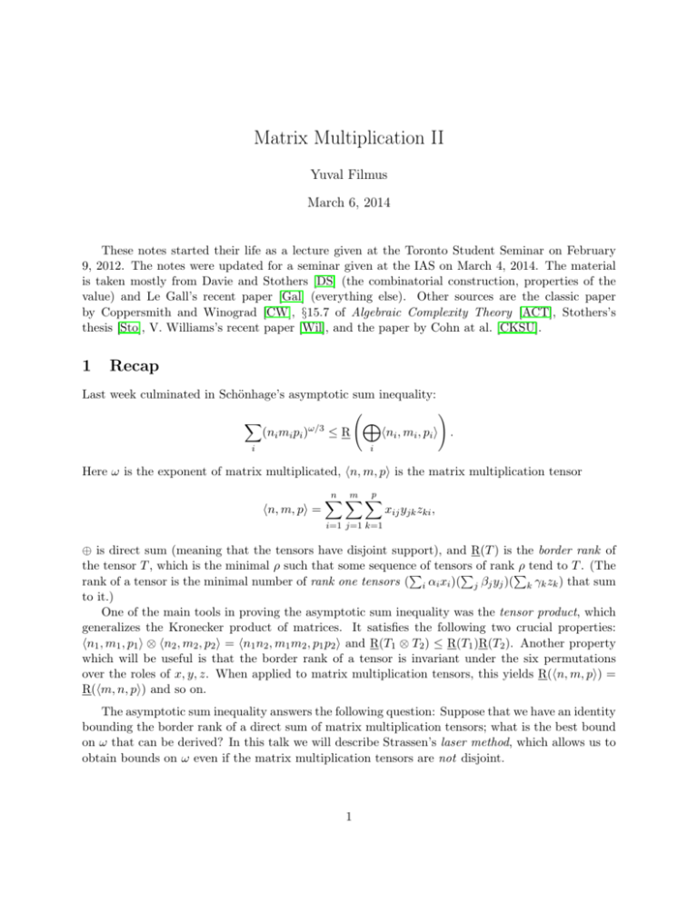
Last week culminated in Schönhage’s asymptotic sum inequality:
X
ω/3
(ni mi pi )
!
M
≤R
hni , mi , pi i .
i
i
Here ω is the exponent of matrix multiplicated, hn, m, pi is the matrix multiplication tensor
hn, m, pi =
p
n X
m X
X
xij yjk zki ,
i=1 j=1 k=1
⊕ is direct sum (meaning that the tensors have disjoint support), and R(T ) is the border rank of
the tensor T , which is the minimal ρ such that some sequence
ρ tend to T . (The
Pof tensors
P of rankP
rank of a tensor is the minimal number of rank one tensors ( i αi xi )( j βj yj )( k γk zk ) that sum
to it.)
One of the main tools in proving the asymptotic sum inequality was the tensor product, which
generalizes the Kronecker product of matrices. It satisfies the following two crucial properties:
hn1 , m1 , p1 i ⊗ hn2 , m2 , p2 i = hn1 n2 , m1 m2 , p1 p2 i and R(T1 ⊗ T2 ) ≤ R(T1 )R(T2 ). Another property
which will be useful is that the border rank of a tensor is invariant under the six permutations
over the roles of x, y, z. When applied to matrix multiplication tensors, this yields R(hn, m, pi) =
R(hm, n, pi) and so on.
The asymptotic sum inequality answers the following question: Suppose that we have an identity
bounding the border rank of a direct sum of matrix multiplication tensors; what is the best bound
on ω that can be derived? In this talk we will describe Strassen’s laser method, which allows us to
obtain bounds on ω even if the matrix multiplication tensors are not disjoint.
1
2
Warmup
We start our exploration with the warmup identity of Coppersmith and Winograd [CW]:
3
q X
[0] [1] [1]
[1] [0] [1]
[1] [1] [0]
x0 yi zi + xi y0 zi + xi yi z0
+ O(4 ) =
i=1
q
X
[0]
[1]
[0]
[1]
[0]
[1]
(x0 + xi )(y0 + yi )(z0 + zi )−
i=1
[0]
x0
(1 −
2
+
q
X
!
[1]
xi
[0]
y0
2
+
q
X
!
[1]
yi
[0]
z0
+
i=1
i=1
[0] [0] [0]
q)x0 y0 z0 .
2
q
X
!
[1]
zi
+
i=1
This identity concerns the following sets of variables:
[0]
[1]
[0]
[1]
[0]
[1]
x0 , x1 , . . . , x[1]
q ,
y0 , y1 , . . . , yq[1] ,
z0 , z1 , . . . , zq[1] .
[0]
We have partitioned the x-variables into two different sets, one consisting of x0 , and the other
[1]
[1]
of x1 , . . . , xq . The y-variables and z-variables are similarly partitioned. We can summarize this
identity as follows:
R(h1, 1, qi0,1,1 + hq, 1, 1i1,0,1 + h1, q, 1i1,1,0 ) ≤ q + 2.
We have annotated each matrix multiplication tensor with the labels of the x-variables, y-variables
and z-variables involved. This tells us, for example, that h1, 1, qi0,1,1 and hq, 1, 1i1,0,1 share zvariables but have disjoint x-variables and y-variables.
We cannot apply the asymptotic sum inequality to this identity, since the matrix multiplication
tensors are not disjoint. Instead, our strategy will be different: we will take a high tensor power
and then zero variables in such a way that the tensors that remain are disjoint, and then apply
the asymptotic sum inequality. We will always zero variables in groups, according to the indices
describing them.
After taking an N th tensor power, we get an identity bounding the border rank of a sum of
3N matrix multiplication tensors by (q + 2)N . The tensors have different formats (dimensions)
hn, m, pi, but the asymptotic sum inequality only cares about their volume (nmp)1/3 , which is the
same for all of them, namely q N/3 . Suppose that we could zero some of the variables so that what
remains is KN disjoint tensors. The asymptotic sum inequality then gives KN q N ω/3 ≤ (q + 2)N or
1/N
KN q ω/3 ≤ (q + 2). How large can KN be?
Each tensor in the N th tensor power involves certain groups of variables. For example, when
[1] [1]
N = 1, the tensor h1, 1, qi0,1,1 involves the variables x[0] , yi , zi . When N = 2, the tensor
h1, 1, qi0,1,1 ⊗ hq, 1, 1i1,0,1 involves the variables
[1]
[1]
[1]
[1]
x[0] ⊗ xj , yi ⊗ y [0] , zi ⊗ zj .
[01]
[10]
[11]
We can write this more concisely as xj , yi , zij , and the tensor itself can be described concisely
as hq, 1, qi01,10,11 . When zeroing variables, we will always zero variables in groups: for example, we
2
[11]
could zero all variables zij . We call these groups x-, y− and z-groups. The annotations themselves
(say 11) we call indices, so the annotation of each tensor is an index triple.
Easy upper bounds. We start with some rather trivial upper bounds on KN . After zeroing out
variables, all the x-groups that remain appear in a unique matrix multiplication tensor. There are
2N different x-groups, so KN ≤ 2N .
A slightly less trivial upper bound on KN , due to Cohn et al. [CKSU], arises from the idea of
source distribution. The set of index triples has the product structure ((0, 1, 1)+(1, 0, 1)+(1, 1, 0))N .
We can decompose this set into typesdepending on how many times each factor was used: for each
N
a, b, c summing to N , there are a,b,c
index triples of type (a, b, c). An x-index in any such triple
contains a zeroes, a y-index contains b zeroes, and a z-index contains c zeroes. There are N 2+2
different types. The source distribution, a scale-invariant quantity, is (a/N, b/N, c/N ).
Consider any type (a, b, c), and assume without loss of generality that a ≤ N/3. Focus on
surviving index
triples
of type (a, b, c). Each such index triple must have a unique x-index, and
N
there are Na ≤ N/3
of these. Accounting for all possible source distributions, we obtain KN ≤
N N +2
N
h(1/3)
. (Here h(p) = −p log2 p − (1 − p) log2 (1 − p) is the binary entropy function.)
N/3 ≈ 2
2
The bound. Surprisingly, this bound is tight! There is a construction achieving KN ≥ 2N h(1/3)−o(N ) .
This implies that 2h(1/3) q ω/3 ≤ (q + 2). Optimizing over q, we find out that when q = 8 we get the
bound ω ≤ 2.404.
3
The Construction
We now describe the construction giving KN ≈ 2N h(1/3) . It will be advantageous to describe it in
greater generality. We start by describing the parameters of the construction, instantiating them
for our present case. First, the basic index set, consisting of triples of integers, which we assume
to be rotation-invariant (with respect to permutations of the three indices), and tight: every basic
index triple sums to the same value. Tightness is crucial for the construction. The basic index set
in our case is
(0, 1, 1), (1, 0, 1), (1, 1, 0).
Second, a rotation-invariant source distribution π, prescribing the type of tensors we’re looking at:
π = (1/3, 1/3, 1/3).
These are the inputs. Given N (the tensor power), we will describe the results in terms of three
quantities P, F, G, defined below. We will use N π to mean the type of an index triple induced by
π, in our case (N/3, N/3, N/3) (we will not worry about these being integers). We are aiming at
index triples of type N π. An x-index has type N π if it appears in an index triple of type N π. An
index triple (i, j, k) has projection type N π if i, j, k all have type N π. In our case, an index triple
(i, j, k) has projection type N π = (N/3, N/3, N/3) if and only if it has type N π, but in some cases
there might be more index triples of projection type N π than index triples of (strict) type N π (see
discussion below). The parameters P, F, G are:
• P is the number of x-indices of type N π. (Because of rotation invariance, it is also the number
of y-indices and z-indices of type N π.)
3
• F is the number of index triples of type N π.
• G is the number of index triples of projection type N π.
The upper bound we described above is P . Our construction will give (F/G)P 1−o(1) , which is tight
when F = G.
The applications below will actually require a slightly more general result: instead of considering
all index triples of projection type N π as possible obstructions, we will allow a pre-filtering step
which eliminates some of them at the outset. In that case, G will be the number of index triples
after the pre-filtering, and what we require is that after zeroing variables, no index repeats in the
pre-filtered index triples.
Mock construction. We start with a mock construction. Suppose that instead of zeroing variables, we are allowed to select index triples, under the constraint that no x-index, y-index or z-index
repeats. In this case, we will be able to achieve Ω(P ) using a very simple construction. We can
focus on index triples of type N π. The idea is to select each index triple with some probability ,
and to filter out bad index triples, which are surviving index triples that have a matching index
with some other surviving index triple. Call the remaining index triples good.
Each index triple (i, j, k) could potentially conflict with 3(F/P − 1) other index triples: symmetry considerations show that there are F/P index triples each of the form (i, ·, ·), of the form
(·, j, ·), and of the form (·, ·, k). Therefore the probability that an index triple is bad is at most
2 3F/P , and the probability that it is good is at least − 2 3F/P . The choice of maximizing this
expression is = P/6F , giving a probability of P/12F . Therefore the expected number of good
index triples is F · (P/12F ) = P/12 = Ω(P ).
The problem. For the actual construction, we need to zero variables rather than eliminate
triples. We start by zeroing all variables other than those of type N π, leaving only index triples of
projection type N π in play (it is this step that will be replaced by a different pre-filtering in some
of the applications). We are going to follow the same basic approach: we select each index triple
of type N π with some probability , and then eliminate bad index triples (these will be defined
in a bit). Following that, we will restrict the variables to those variables appearing in good index
triples. This gives us a set of resulting index triples, those index triples all whose variables have
survived. We want this set to have no repeated x-, y- or z-indices.
We will define bad index triples in such a way that no index repeats in the good index triples.
But this doesn’t guarantee that the resulting index triples have no repeated indices. We could have
the following situation:
i1
j1
k1
i2
j2
k2
i3
j3
k3
Here (i1 , j1 , k1 ), (i2 , j2 , k2 ), (i3 , j3 , k3 ) are good index triples, and the diagonal (i1 , j2 , k3 ) is a potential resulting index triple that conflicts with them. (This should remind the knowledgeable reader
of the uniquely solvable puzzles (USPs) in Cohn et al. [CKSU].) Notice that while the former index
triples have type N π, the diagonal (i1 , j2 , k3 ) is only known to have projection type N π.
Given the first index triple (i1 , j1 , k1 ), there are G/P choices for j2 , k3 , and then F/P choices
each for i2 , k2 and i3 , j3 . If we define a bad index triple as one which participates in such a constellation, then the probability that an index triple is good is at least − 3F/P 2 − 3GF 2 /P 3 3 (going
4
over all possible choices of the common index). For simplicity, remove the term 3F/P 2 from this
expression. The choice of maximizing the expression − 3GF 2 /P 3 3 is = P 3/2 /3G1/2 F , giving
a probability of 2P 3/2 /9G1/2 F , and an expected number of resulting triples which is 2P 3/2 /9G1/2 .
1/2
n 3/2
n
n
In our running example, P 3/2 /G1/2 = n/3
/ n/3,n/3,n/3
≈ 2n(log2 3−1) , whereas P = n/3
≈
2n(log2 3−2/3) . In other words, the bound is not asymptotically tight.
The trick. The idea is to come up with a way of choosing the initial index triples with the
following property. In the situation described above, if (i1 , j1 , k1 ), (i2 , j2 , k2 ), (i3 , j3 , k3 ) are all
selected, then so is (i1 , j2 , k3 ). This means that our method of choosing index triples will choose
not only index triples of type N π but also index triples of projection type N π; we will only be
interested in the number of resulting index triples of (strict) type N π. In order to guarantee that
no bad constellation arises, it will be enough to guarantee that all the chosen index triples will have
distinct indices. Retracing our footsteps, we expect that an index triple be good with probability
roughly − 2 3G/P , assuming that our method of choosing index triples is 2-wise independent
(at least approximately). Optimizing over , this probability should be roughly P/6G, and so the
number of good index triples of (strict) type N π should be around (F/6G)P in expectation.
We now reach the surprising part of the construction, which is the new method of choosing index
triples. Let M be a large prime roughly equal to 1/. We will define three random hash functions
hx , hy , hz mapping the individual indices to ZM . For some appropriately defined set A ⊆ ZM of
cardinality M 1−o(1) , we will choose all index triples (i, j, k) such that hx (i), hy (j), hz (k) ∈ A. Our
random hash functions and set A will be chosen so that the following properties hold:
(P1) For all x-indices i1 and y-indices j1 6= j2 , the hash triple (hx (i1 ), hy (j1 ), hy (j2 )) is distributed
uniformly over Z3M . (And similarly for all other choices of positions among x, y, z.)
(P2) For all index triples (i, j, k),
hx (i), hy (j), hz (k) ∈ A if and only if hx (i) = hy (j) = hz (k) ∈ A.
(P3) For all index triples (i, j, k), if any two of hx (i), hy (j), hz (k) are equal then all are equal.
Given these properties, we show how to complete the proof. An index triple (i1 , j1 , k1 ) is chosen if
for some a ∈ A, hx (i1 ) = hy (j1 ) = hz (k1 ) = a, or equivalently hx (i1 ) = hy (j1 ); this happens with
probability |A|M −2 = M −1−o(1) = 1+o(1) . A chosen index triple (i1 , j1 , k1 ) is bad if it shares an
index with another chosen index triple. There are at most 3G/P such index triples which could
conflict with (i1 , j1 , k1 ). A pair of conflicting index triples, say (i1 , j1 , k1 ) and (i1 , j2 , k2 ), are both
chosen if for some a ∈ A, hx (i1 ) = hy (j1 ) = hy (j2 ) = a. This happens with probability |A|M −3 =
M −2−o(1) = 2+o(1) . Hence an index triple is good with probability at least 1+o(1) − (3G/P )2+o(1) ,
which for an appropriate choice of becomes (P/G)1−o(1) . So the expected number of good triples
of (strict) type N π is F (P/G)1−o(1) ≥ (F/G)P 1−o(1) . As commented above, the resulting index
triples have no repeated indices, completing the proof.
Defining the hash function. We will construct hx , hy , hz so that for all index triples i, j, k,
hx (i) + hy (j) = 2hz (k) (property P4). We will be able to guarantee this property since the basic index triples are tight by assumption: all indices sum to the same constant, which without
loss of generality is zero. This already shows that for every index triple (i, j, k), if any two of
5
hx (i), hy (j), hz (k) are equal, then all are equal (property P3). Property P2 would hold exactly
if A contains no three-term arithmetic progressions other than constant ones. We’re very lucky
that Salem and Spencer [SS] constructed such a set for us of size M 1−o(1) . (Better constructions
exist [Beh, Mos, Elk], but the difference doesn’t matter here.) It is now a simple exercise to define
hx , hy , hz so that properties P1 and P4 are satisfied: let α ∈ ZN
M and X, Y, Z ∈ ZM be chosen
randomly under the constraint X + Y + Z = 0, and define (over ZM )
hx (i) = 2(hα, ii + X),
hy (j) = 2(hα, ji + Y ),
hz (k) = −(hα, ki + Z).
To see that property P4 holds, use i + j + k = 0 to get
hx (i) + hy (j) = 2(hα, i + ji + X + Y ) = −2(hα, ki + Z) = 2hz (k).
To see that property P1 holds, let D = j2 − j1 6= 0. We have
1
2 (hx (i1 ), hy (j1 ), hy (j2 ))
= (hα, i1 i + X, hα, j1 i + Y, hα, j1 i + Y + hα, Di).
The three quantities X, Y, hα, Di are distributed uniformly in Z3M , implying that property P1 holds.
Strassen’s version. Strassen [S2] came up with an alternative construction which trades Salem–
Spencer sets for tensor degeneration. This is the process in which, in addition to zeroing some of
the variables, we multiply the rest by some powers of , the result being those tensors with the
minimal coefficient of . This gives an upper bound on the border rank of the adjusted tensor, and
we can apply the asymptotic sum inequality as before. We start by zeroing all variables other than
those of projection type N π. We then multiply variables according to the hash of their index, as
follows:
2
x[i] → 2hx (i) ,
2
y [j] → 2hy (j) ,
2
z [k] → −4hz (k) .
Here we think of the hashes as integers in {0, . . . , M − 1} rather than elements of ZM . The analog
of property P2 is this: an index triple (i, j, k) has minimal power if and only if hx (i) = hy (j) =
hz (k) ∈ B, where B ⊆ {0, . . . , M − 1} will turn out to have size Ω(M ) (rather than just M 1−o(1) ).
What is the power corresponding to a tensor with index triple (i, j, k)? Recall that hx (i) +
hy (j) ≡ 2hz (k) (mod M ). The left-hand side is strictly smaller than 2M , and so there are two
cases: either 2hz (k) = hx (i) + hy (j) or 2hz (k) = hx (i) + hy (j) − M . In the first case, the exponent
of is
2hx (i)2 + 2hy (j)2 − (2hz (k))2 = 2hx (i)2 + 2hy (j)2 − (hx (i) + hy (j))2 = (hx (i) − hy (j))2 .
In the second case, the exponent of is
2hx (i)2 + 2hy (j)2 − (2hz (k))2 = 2hx (i)2 + 2hy (j)2 − (hx (i) + hy (j) − M )2
= (hx (i) − hy (j))2 + M (2hx (i) + 2hy (j) − M ) ≥ M 2 .
We conclude that the minimum power of is attained at index triples (i, j, k) satisfying hx (i) = hy (j)
and 2hx (i) < M , that is, hx (i) = hy (j) = hz (k) ∈ B = {0, . . . , (M − 1)/2}, where |B| > |M |/2.
6
Strassen’s identity. Strassen [S1] originally came up with this method of tensoring followed by
zeroing (or degeneration) in the context of another identity:
q
X
[1] [0] [1]
[0] [1] [1]
(xi y0 zi + x0 yi zi ) + O(2 ) =
i=1
q
X
[0]
[1]
[0]
[1]
[0] [0]
(x0 + xi )(y0 + yi )zi − x0 y0
i=1
q
X
zi .
i=1
This identity shows that R(hq, 1, 1i1,0,1 + h1, 1, qi0,1,1 ) ≤ q + 1. Strassen used a direct construction
showing 4q ω ≤ (q + 1)3 , which for q = 5 gives ω < 2.48. See Strassen’s original paper or §15.6
of [ACT] for details.
Tightness of the construction. So far we have only considered one application of the construction, in which G = F . As we remarked above, when G = F the construction is optimal in the
1/N
sense that it achieves the best possible limN →∞ KN under the given combinatorial constraints.
However, in some cases G 6= F . This can happen when there are two rotation-invariant source
distributions whose projections to the x-index are the same. Here is an example:
Index triple Probability
(0, 3, 3)
1/9
(3, 0, 3)
1/9
(3, 3, 0)
1/9
(1, 1, 4)
1/9
1/9
(1, 4, 1)
(4, 1, 1)
1/9
(2, 2, 2)
1/3
Index triple Probability
(0, 2, 4)
1/9
1/9
(2, 4, 0)
(4, 0, 2)
1/9
(1, 2, 3)
2/9
(2, 3, 1)
2/9
(3, 1, 2)
2/9
The projections to the x-index are both
x-index Probability
0
1/9
1
2/9
2
1/3
3
2/9
1/9
4
This is the smallest example in the sense that there is no such example with only {0, 1, 2, 3}.
For given N , the answer lies somewhere between P and (F/G)P 1−o(1) . We can
P estimate these
quantities asymptotically. It is well-known that F ≈ 2N H(π) , where H(π) = − i π(i) log2 π(i) is
the binary entropy function, and the approximation is up to polynomial terms P
(in N ). Similarly,
if πx is the projection of π into the x-index, then P ≈ 2N H(πx ) . Finally, G ≈ σ : πx =σx 2N H(σ) ,
for all source distributions σ realizable exactly on N coordinates, that is, each probability is an
integer multiple of 1/N . There are only polynomially many of these, and so we can approximate
G by the maximal one. As N tends to infinity, we can disregard the realizability constraint and
consider arbitrary distributions, and so G ≈ maxσ : πx =σx 2N H(σ) , where σ now is any probability
distribution (technically this should be a supremum, but it is easy to check that the supremem is
7
always achieved). In fact, the concavity of the entropy function shows that the maximizing σ must
be rotation-invariant. Putting everything together, we get the following bounds:
1/N
H(πx ) + H(π) − max H(σ) ≤ log2 lim KN
σ : σx =πx
N →∞
≤ H(πx ).
1/N
(It is not hard to check that KN1 N2 ≥ KN1 KN2 , implying that the limit limN →∞ KN
exists.)
This leads to the following open question.
in fact
1/N
Open question 1. What is the best possible limN →∞ KN achievable given basic index triples
and a source distribution? Does using degeneration (see Strassen’s version above) lead to better
results?
We conjecture that the construction is optimal.
4
A better identity
The identity considered up to now can be slightly tweaked to yield even more:
"
3
q X
[0] [1] [1]
x 0 yi z i
+
[1] [0] [1]
xi y0 zi
+
[1] [1] [0]
xi yi z0
#
+
[0] [0] [2]
x0 y0 zq+1
+
[0] [2] [0]
x0 yq+1 z0
+
[2]
[0] [0]
xq+1 y0 z0
+ O(4 ) =
i=1
q
X
[0]
[1]
[0]
[1]
[0]
[1]
(x0 + xi )(y0 + yi )(z0 + zi )−
i=1
[0]
x0
(1 −
2
+
q
X
!
[1]
xi
[0]
y0
2
+
i=1
[0]
[2]
[0]
q)(x0 + 3 xq+1 )(y0
+
q
X
!
[1]
yi
i=1
[0]
3 [2]
yq+1 )(z0
[0]
z0
+
2
+
q
X
!
[1]
zi
+
i=1
3 [2]
zq+1 ).
This shows that
R(h1, 1, qi0,1,1 + hq, 1, 1i1,0,1 + h1, q, 1i1,1,0 + h1, 1, 1i0,0,2 + h1, 1, 1i0,2,0 + h1, 1, 1i2,0,0 ) ≤ q + 2.
The new factors h1, 1, 1i come at absolutely no cost! In fact, more can be added in the same way,
but this doesn’t result in any further improvement.
In contrast with the previous identity, the basic index triples here have different volumes (recall
that the volume of hn, m, pi is (nmp)ω/3 ). For a given (rotation-invariant) source distribution
π = (α/3, α/3, α/3, β/3, β/3, β/3), the volume of each of the corresponding tensors in the N th
tensor power of the basic identity is q (α/3)N . The corresponding distribution of x-indices is π1 =
(α/3 + 2β/3, 2α/3, β/3), from which we can recover π; this shows that we can recover π from π1 (as
long as we are restricted to rotation-invariant distributions), and so G = F in the combinatorial
construction. The combinatorial construction therefore shows how to zero variables so as to obtain
TN tensors, where TN ≈ 2H(π1 )N . Feeding this to the asymptotic sum inequality, we obtain
2H(α/3+2β/3,2α/3,β/3) q (α/3)ω ≤ q + 2.
For each given value of q, we can minimize ω over the choice of α + β = 1 numerically (we will
describe how this can be done systematically later on). We find out that the smallest value of ω is
obtained for q = 6 and α ≈ 0.952, which gives the bound ω ≤ 2.388.
8
5
Milking the identity
All further improvements rely on the same identity just analyzed, dating to the STOC ’87 paper
if not earlier. How can this identity yield better bounds? So far we have considered the following
process: starting with the basic identity, take a high tensor power, zero some of the variables so that
whatever remains is a collection of disjoint matrix multiplication tensors, and apply the asymptotic
sum inequality. We can improve on this by allowing non-disjoint matrix multiplication tensors,
assuming that we can merge them together1 . For example, consider the two tensors
h1, 1, q1 ii,j1 ,k1 =
h1, 1, q2 ii,j2 ,k2 =
q1
X
t=1
q2
X
[j ] [k1 ]
,
[j ] [k2 ]
,
x[i] yt 1 zt
x[i] yt 2 zt
t=1
having an identical x-index. If we sum them together then we get the tensor
!
q1
q2
X
X
[j ] [k ]
[j ] [k ]
x[i]
yt 1 zt 1 +
yt 2 zt 2 ,
t=1
t=1
which is simply a manifestation of h1, 1, q1 + q2 i. Without this merging, we can only keep one of the
tensors above. With this merging, we can pick both of them together, though the merged version
ω/3
ω/3
is not worth as much as two separate ones since (q1 + q2 )ω/3 < q1 + q2 (assuming ω < 3). We
ω/3 ω/3
gain since (q1 + q2 )ω/3 > max(q1 , q2 ).
One principled way of applying this idea is by merging tensors as soon as possible: we take
a small tensor power of the basic identity, merge some tensors, and then apply the construction.
After taking the small tensor power, each index is now a vector of integers. However, for the
combinatorial construction to work, we need integer indices whose sum is constant. One natural
choice of such “coupling” is by letting the new index be the sum of the vector of indices. This
folds some of the tensors together. When the folded tensors can be put together into one larger
matrix multiplication tensor, we have gained something. However, the sum could also be a new
kind of tensor which isn’t a matrix multiplication tensor. We will handle such tensors by applying
the construction recursively.
The smallest tensor power that can be considered is the square, and this case has been considered
already by Coppersmith and Winograd. Successively larger power have been considered by other
authors: Stothers [Sto, DS] considered the fourth power, Vassilevska-Williams [Wil] considered
(independently) the fourth and eighth powers, and very recently Le Gall [Gal] considered the
sixteenth and thirty-second power. The following table, taken from Le Gall’s paper, summarizes
the results obtained in this way:
Who
Power
Bound
C.-W.
1
ω < 2.3871900
C.-W.
2
ω < 2.3754770
Stothers
4
ω < 2.3729269
V.-Williams
8
ω < 2.3728642
Le Gall
16
ω < 2.3728640
Le Gall
32
ω < 2.3728639
1
We thank Andris Ambainis for this observation.
9
6
Squared identity
We start by considering the simplest case, the square of the basic identity:
R((h1, 1, qi0,1,1 + hq, 1, 1i1,0,1 + h1, q, 1i1,1,0 + h1, 1, 1i0,0,2 + h1, 1, 1i0,2,0 + h1, 1, 1i2,0,0 )2 ) ≤ (q + 2)2 .
Opening up the square, we get 36 terms on the left-hand side, starting with h1, 1, qi0,1,1 ⊗h1, 1, qi0,1,1 =
h1, 1, q 2 i00,11,11 . Each of these 36 terms are matrix multiplication tensors. In order to apply the combinatorial edifice, we will need to divide the new variables into groups with integer indices, in such a
way that the indices in each tensor add up to the same number. One way of doing this is by putting
variables x[i1 ,i2 ] in group i1 + i2 , and so on: this guarantees that the sum is always 4. Continuing
our example, the variables in h1, 1, q 2 i00,11,11 are now going to belong to the groups 0, 2, 2. There
are two other tensors whose new grouping will be 0, 2, 2: h1, 1, 1i0,2,0 ⊗ h1, 1, 1i0,0,2 = h1, 1, 1i00,20,02
and h1, 1, 1i0,0,2 ⊗ h1, 1, 1i0,2,0 = h1, 1, 1i00,02,20 . Notice that all these three tensors share the same
x variable, but otherwise the variables are disjoint. Therefore we can merge all three of them to a
tensor h1, 1, q 2 + 2i0,2,2 .
By employing a similar analysis to all the terms, we come up with the following terms:
(a) 3 terms similar to h1, 1, 1i0,0,4 , coming from
h1, 1, 1i0,0,2 ⊗ h1, 1, 1i0,0,2 .
(b) 6 terms similar to h1, 1, 2qi0,1,3 , coming from
h1, 1, qi0,1,1 ⊗ h1, 1, 1i0,0,2 ⊕ h1, 1, 1i0,0,2 ⊗ h1, 1, qi0,1,1 .
(c) 3 terms similar to h1, 1, q 2 + 2i0,2,2 , coming from
h1, 1, 1i0,2,0 ⊗ h1, 1, 1i0,0,2 ⊕ h1, 1, 1i0,0,2 ⊗ h1, 1, 1i0,2,0 ⊕ h1, 1, qi0,1,1 ⊗ h1, 1, qi0,1,1 .
(d) 3 terms similar to T41,1,2 , coming from
h1, q, 1i1,1,0 ⊗h1, 1, 1i0,0,2 +h1, 1, 1i0,0,2 ⊗h1, q, 1i1,1,0 +hq, 1, 1i1,0,1 ⊗h1, 1, qi0,1,1 +h1, 1, qi0,1,1 ⊗hq, 1, 1i1,0,1 .
There is a problem here: if we group together all terms involving the new groups 1, 1, 2, we don’t
get a matrix multiplication tensor, but rather
T4 = h1, q, 1i10,10,02 + h1, q, 1i01,01,20 + hq, 1, qi10,01,11 + hq, 1, qi01,10,11 .
There are two other terms ρ(T4 ), ρ2 (T4 ) similar to T4 which differ only by rotation of the indices.
(In general, the operator ρ rotates the tensor by applying the transformation (x, y, z) 7→ (y, z, x);
for example ρ(hn, m, pi) = hm, p, ni.) We have retained the original indices to show which variables
are the same and which are disjoint. We can retain the same information by considering just the
first half of each index, because the two halves sum to a constant. The result is
T4 = h1, q, 1i1,1,0 + h1, q, 1i0,0,2 + hq, 1, qi1,0,1 + hq, 1, qi0,1,1 .
The indices now sum to the original value 2.
10
Following the recipe, we should now take a high tensor power, zero some variables, and use the
asymptotic sum inequality to get a bound on ω. This will be problematic since T4 is not a matrix
multiplication tensor: after zeroing the variables, we will have terms of the form hn, m, pi ⊗ T4q ⊗
ρ(T4 )q ⊗ ρ2 (T4 )q (ostensibly, the three tensors T4 , ρ(T4 ), ρ2 (T4 ) could have different powers, but this
does not happen since the source distribution we choose is always rotation-invariant). The idea
now is to zoom in on (T4 ⊗ρ(T4 )⊗ρ2 (T4 ))q , and zero variables so that disjoint matrix multiplication
tensors are obtained. We already know how to do this: just apply the very same construction that
got us here!
Value of a tensor. We now formalize this idea through the notion of value, which is what a
given tensor gives you in view of applying the asymptotic sum inequality. Our goal is to generalize
the asymptotic sum inequality to
X
M
Vω (Ti ) ≤ R(
Ti ).
i
i
If all tensors Ti are matrix multiplication tensors Ti = hni , mi , pi i, then putting Vω (Ti ) = (ni mi pi )ω/3
recovers the asymptotic sum inequality.
We define the value of a tensor in two steps. Suppose
first that T is rotation-invariant: T = ρ(T ).
P
For each N , we define Vω,N as the maximum of i (ni mi pi )ω/3 over all ways of zeroing variables to
L
1/N
obtain i hni , mi , pi i from T ⊗N . It is easy to check that Vω,N1 N2 ≥ Vω,N1 Vω,N2 , and so Vω,N tends
to a limit, which is the value Vω (T ).
When T is not rotation-invariant, we define Vω (T ) = (Vω (T ⊗ ρ(T ) ⊗ ρ2 (T )))1/3 . When T is
rotation-invariant, both definitions coincide. The reason we consider T ⊗ ρ(T ) ⊗ ρ2 (T ) is that the
tensor T in fact appears in such a fashion in the construction, as we hinted above.
The generalized asymptotic sum inequality. The proof of the generalized asymptotic sum
inequality isn’t too hard. We start with a preliminary result.
L
Lemma 1. For any two tensors T1 , T2 , Vω (T1 ⊗ T2 ) ≥ Vω (T1 )Vω (T2 ) and Vω (T1 T2 ) ≥ Vω (T1 ) +
Vω (T2 ).
Proof. The first part follows from the simple observation Vω,N (T1 ⊗ T2 ) ≥ Vω,N (T1 )Vω,N (T2 ).
For the second part, assume for simplicity that the tensors T1 , T2 are rotation-invariant: otherwise, the symmetrized tensors Ti ⊗ ρ(TiL
) ⊗ ρ2 (Ti ) should be considered instead. For every two
rotation-invariant tensors S1 , S2 , Vω,N (S1 S2 ) = Vω,N (S1 ) + Vω,N (S2 ). Therefore
X N Vω,N (T1 + T2 ) ≥
Vω,N1 (T1 )Vω,N2 (T2 ).
N1
N1 +N2 =N
When N1 , N2 are large, which accounts for most of the sum, Vω,N1 (T1 ) ≈ Vω (T1 )N1 and Vω,N2 (T2 ) ≈
Vω (T2 )N2 , and so the binomial theorem gives Vω,N (T1 + T2 ) ≈ (Vω (T1 ) + Vω (T2 ))N .
This argument can be formalized; the only step we need to justify is that large N1 , N2 account
for most of the sum. Indeed, the largest term in the sum accounts for a polynomial fraction of the
sum, and this term is the one satisfying N1 /N2 ≈ Vω (T1 )/Vω (T2 ). Assuming the values are non-zero,
this shows that a polynomial fraction of the sum is concentrated at a term with N1 , N2 = Ω(N ).
11
In order to prove the generalized asymptotic sum inequality, it will be more convenient to state
the asymptotic sum inequality in the following equivalent form:
M
X
Ti ) =⇒ ω ≤ α,
(ni mi pi )α/3 ≥ R(
i
i
L
and prove a similar statement for the value. Let T = i Ti and S = T ⊗ ρ(T ) ⊗ ρ2 (T ). Suppose
that
X
Vα (Ti ) ≥ R(T ).
i
The lemma shows that Vα (T ) ≥ R(T ), and so for large N ,
Vα,N (S) & Vα (S)n = Vα (T )3n ≥ R(T )3N ≥ R(S)N .
The asymptotic inequality immediately implies that ω . α. In the limit, we obtain ω ≤ α.
Lower bounding the value of a tensor. Having shown how the value can be used to deduce
upper bounds on ω, we proceed to interpret the combinatorial construction as a lower bound on
the value. When T = hn, m, pi, we immediately get Vω (T ) ≥ (nmp)ω/3 (in fact there is equality).
Suppose now that we have a tensor of the form
X i ,j ,k
T =
Tt t t t .
t
Each individual tensor Ttit ,jt ,kt is supported by x-variables having the (integer) index it , y-variables
having the index jt , and zt -variables having the index k. The crucial property of the indices is that
for it 6= is , the x-variables having index it are disjoint from the x-variables having index is . We
also need the index triples to be tight: it + jt + kt must be a constant independent of t.
Suppose first that T is rotation-invariant. We need to estimate Vω (T ). The definition of
value easily implies that Vω (T ) = Vω (T ⊗N )1/N . For each source distribution π, the combinatorial
construction shows that starting with T ⊗N , there is a way of zeroing variables so as to obtain KN
N ⊗N π(t)
, where KN ≈ 2N κ for
copies the tensor t Tt
κ = H(πx ) + H(π) − max H(σ).
σ : σx =πx
(Recall that πx is the projection of π into the x-index.) Since the value is super-additive and
super-multiplicative, this shows that
Y
Vω (T )N = Vω (T ⊗N ) & 2N κ
Vω (Tt )N π(t) .
t
Therefore for each source distribution π, we obtain the following bound on Vω (T ):
X
log2 Vω (T ) ≥ H(πx ) + H(π) − max H(σ) +
π(t) log2 Vω (Tt ).
σ : σx =πx
t
Maximizing this over π (a process which we address later on) gives us a lower bound on Vω (T ).
When T is not rotation-invariant, the definition requires us to examine S = T ⊗ ρ(T ) ⊗ ρ2 (T )
instead. Every source distribution π for T lifts naturally to a source distribution π S on S, given by
12
π S (t1 , t2 , t3 ) = π(t1 )π(t2 )π(t3 ) (here it is important to use the same indexing for the constituent
tensors of T, ρ(T ), ρ2 (T )). It is easy to check that H(π S ) = 3H(π) and H(πxS ) = H(πx ) + H(πy ) +
H(πz ). Similarly,
X
π S (t1 , t2 , t3 ) log2 Vω (Tt1 ⊗ ρ(Tt2 ) ⊗ ρ2 (Tt3 ))
t1 ,t2 ,t3
X
≥
π(t1 )π(t2 )π(t3 )(log2 Vω (Tt1 ) + log2 Vω (Tt2 ) + log2 Vω (Tt3 ))
t1 ,t2 ,t3
=3
X
π(t) log2 Vω (Tt ).
t
One last thing we need to determine is when a distribution σ S satisfies σxS = πxS . Suppose for the
moment that we only considered lifted distributions. In that case, it is not hard to check that the
requied condition is σx = πx , σy = πy and σz = πz , which we summarize by writing σ ≡ π, in
words, σ is compatible with π. Assuming this, we get the lower bound
log2 Vω (T ) =
X
H(πx ) + H(πy ) + H(πz )
1
log2 Vω (S) ≥
+ H(π) − max H(σ) +
π(t) log2 Vω (Tt ).
σ≡π
3
3
t
Unfortunately, while this lower bound indeed holds, its proof is slightly more complicated, involving
a pre-filtering step. Instead of taking an N th tensor power of S, we take an N th tensor power of T ,
and zero out all variables other than those having projection type N π, obtaining a tensor T 0 . The
number of index triples having projection type N π is roughly maxσ≡π 2N H(σ) . We then consider
the tensor S 0 = T 0 ⊗ρ(T 0 )⊗ρ2 (T ), which can be obtained from S by zeroing out variables. All index
triples have projection type N 3 π S , and their number is approximately 23N H(σ) . The construction
now applies, and gives the stated lower bound.
Wrapping things up. For each value of α, we can now obtain a lower bound on Vα (T4 ), since all
the component tensors Tt are matrix multiplication tensors and so have known value. In fact, we
can solve the required optimization explicitly, obtaining the lower bound 41/3 q α (2 + q 3α )1/3 . Given
Vα (T4 ), we can now optimize over the value of the folded squared identity. If the resulting value is
at least (q + 2)2 , then ω ≤ α. Using binary search, we can find the best bound on ω that can be
obtained in this way, which is ω ≤ 2.376, obtained for q = 6.
7
Optimizing the value lower bound
Our work so far culminated with the following lower bound on the value:
log2 Vα (T ) ≥
X
H(πx ) + H(πy ) + H(πz )
+ H(π) − max H(σ) +
π(t) log2 Vα (Tt ).
σ≡π
3
t
Fix α, and suppose we have somehow calculated Vα (Tt ). It remains to maximize the right-hand
side of the inequality. We start by analyzing the condition σ ≡ π. Let the index triples in question
be (it , jt , kt ), and suppose that the possible values for i, j, k are X, Y, Z (respectively). We can write
13
the condition σ ≡ π as a linear system:
X
(σ(t) − π(t)) = 0
for all x ∈ X,
t : it =x
X
(σ(t) − π(t)) = 0
for all y ∈ Y,
(σ(t) − π(t)) = 0
for all z ∈ Z,
t : jt =y
X
t : kt =z
X
(σ(t) − π(t)) = 0.
t
This is a linear system in σ(t) − π(t). The easy case is when this linear system has no non-trivial
solutions. This happens, for example, when computing Vα (T4 ) and when computing the value of
the folded squared identity. In this case, we can write
log2 Vα (T ) ≥
H(πx ) + H(πy ) + H(πz ) X
+
π(t) log2 Vα (Tt ).
3
t
We want to maximize the right-hand side under the constraint that π is a probability distribution.
Since the entropy function is concave, this is a convex optimization program, which can be solved
efficiently using known methods such as gradient descent.
When the linear system in σ(t) − π(t) has non-trivial solutions, we are not so lucky. In fact, it
seems hard to compute the exact maximum. Instead, Stothers/Vassilevska-Williams [Sto, Wil] and
Le Gall [Gal] offer two different methods to compute good lower bounds, which seem to perform
quite well in practice. Both methods are optimal when the linear system has no non-trivial solutions.
Le Gall’s method. While appearing after the other method, Le Gall’s method is simpler and
much more efficient. He suggests first computing
π ∗ = argmax
π
H(πx ) + H(πy ) + H(πz ) X
+
π(t) log2 Vα (Tt ),
3
t
and then computing
σ ∗ = argmax H(σ).
σ≡π ∗
Both maximizations are convex optimization programs, and so can be solved efficiently. The resulting lower bound is
log2 Vα (T ) ≥
X
H(πx∗ ) + H(πy∗ ) + H(πz∗ )
+ H(π ∗ ) − H(σ ∗ ) +
π ∗ (t) log2 Vα (Tt ).
3
t
Stothers/Vassilveska-Williams’ method. The idea of this method is to add the constraint
π = argmaxσ≡π H(σ). We can express this constraint using Lagrange multipliers. Let V be
the space of solutions of the linear system considered above. Given π, we want π to be a local
maximum of H(π) in a small neighborhood of the form H(π + V ); concavity of H implies that a
local maximum is in fact a global maximum. This means that ∇H(π) ∈ V ⊥ . Since ∇H(π) is the
14
vector −1 − log π(t) and the all one vector is in V ⊥ , this condition can be stated as (log π(t)) ∈ V ⊥ .
(We are skipping a small technicality here, showing that all relevant probabilities must be positive
so that this condition is well-defined.) The resulting optimization program is
max
π : (log π(t))∈V ⊥
H(πx ) + H(πy ) + H(πz ) X
+
π(t) log2 Vα (Tt ).
3
t
This is not a convex optimization program, but can nevertheless be solved in practice using nonlinear solvers. Compared to Le Gall’s method, this method tends to give slightly better lower
bounds on values, but runs much slower since the optimization problem that needs to be solved is
more complicated.
8
Higher powers
It is time now to consider higher powers of the basic identity. Empirically it seems that it is best to
consider powers which are themselves powers of two. The idea is to iterate the squaring operation,
computing the values of all the tensors encountered along the way. For example, consider the
squared identity, which has tensors of the forms h1, 1, 1i0,0,4 , h1, 1, 2qi0,1,3 , h1, 1, q 2 + 2i0,2,2 , T41,1,2 ,
and their rotations. Squaring the squared identity, we can couple the indices again, and consider
the folded tensor. Most of the tensors appearing in the new expression are complicated, but can
be analyzed by calculating lower bounds on their values, since we already know the values of the
constituent tensors. The advantage we gain is by merging some matrix multiplication tensors to
larger matrix multiplication tensors.
In the case of the identity squared, the tensors h1, 1, 2qi0,1,3 and h1, 1, q 2 + 2i0,2,2 resulted from
such merging. Similarly, every index triple of the form (0, ·, ·) comes from tensor products of the form
h1, 1, ·i0,·,· × h1, 1, · · ·i0,·,· , and so just like before, these can be merged. Vassilevska-Williams [Wil]
calculates that for an index triple (0, b, 2r+1 − b), this merging results in a matrix multiplication
tensor h1, 1, Bi for
X
2r !
B=
qe.
b−e
b+e
r
e!( 2 )!(2 − 2 )!
e∈{0,...,b}
e≡b
(mod 2)
For each α, given the values Vα for all the tensors appearing in the new expression (which can be
calculated using the values of their constituent tensors), we can calculate the value of the entire
expression. Using binary search, we find α such that this value exceeds (q + 2)4 , and this gives an
upper bound on ω. For q = 6, we obtain ω < 2.374 this way. This process can be repeated to
obtain even better bounds on ω, resulting in the bounds reported above.
Open question 2. What is the bound on ω obtained by taking the limit of this construction?
We suspect that there is a different way of obtaining this limiting bound that combines tensors
directly rather than by merging tensors in a small tensor power of the basic identity.
Open question 3. Are there other identities giving better bounds on ω?
Computer search might be helpful here.
15
References
[ACT] Peter Bürgisser, Michael Clausen and M. Amin Shokrollahi, Algebraic Complexity Theory,
Springer, 1997.
[Beh] Felix Behrend, On sets of integers which contain no three terms in arithmetic progression,
Proc. Nat. Acad. Sci. 32:331–332, 1946.
[Elk] Michael Elkin, An improved construction of progression-free sets, Israeli J. Math. 184:93–128,
2011.
[CKSU] Henry Cohn, Robert Kleinberg, Balázs Szegedy and Chris Umans, Group-theoretic algorithms for matrix multiplication, FOCS 2005.
[CW] Dan Coppersmith and Shmuel Winograd, Matrix multiplication via arithmetic progressions,
J. Symb.Comput. 9(3):251–280, 1990.
[DS] A. M. Davie and A. J. Stothers, Improved bound for complexity of matrix multiplication,
Proc. Roy. Soc. Edinburgh 143A:351–370, 2013.
[Gal] François Le Gall, Powers of tensors and fast matrix multiplication, arXiv:1401.771, 2014.
[Mos] Leo Moser, On non-averaging sets of integers, Canad. J. Math. 5:245–253, 1953.
[SS] Raphaël Salem and Donald Spencer, On sets of integers which contain no three in arithmetic
progressions, Proc. Nat. Acad. Sci. 28:561–563, 1942.
[Sto] Andrew James Stothers, On the complexity of matrix multiplication, Ph.D. thesis (U. of
Edinburgh), 2010.
[S1] Volker Strassen, The asymptotic spectrum of tensors, Crelles J. Reine Angew. Math. 384:102–
152, 1988.
[S2] Volker Strassen, Degeneration and complexity of bilinear maps: some asymptotic spectra,
Crelles. J. Reine Angew. Math. 413:127–180, 1991.
[Wil] Virginia Vassilevska-Williams, Breaking the Coppersmith-Winograd barrier, STOC 2012.
16