Chapter 4
Introduction to population genetics
§4.1 Hardy-Weinberg Law
First we introduce a minimum of the terminology and mechanisms of population
genetic systems. Chromosomes—usually found in the nucleus—mostly govern the
inheritable characteristics of an organism, Chromosomes may occur singly (the haploid
case) as in some fungi, in pairs (the diploid case), as in mammals, or in large groups
(triploid, tetraploid, in general polyploid) as in many plants. The associated pairs,
triplets, etc., of chromosomes are called homologous. Locus is the position at which a
gene (a sort of unit of the chromosome) occurs on a chromosome. Alleles are alternate
gene forms at given locus. Genotypes are the various possible combinations of alleles
at corresponding loci on homologous chromosomes. In the diploid case if the alleles are
A and a , the genotypes are AA , Aa , and aa .
The population to be considered here, unless specified otherwise, contain diploid
individuals. We concentrate our attention, for the most part, on characters determined by
one or two loci, on a given pair of chromosomes. We usually assume that two
alternative genes (alleles) may occur at each locus. Consider the case of two loci, where
the alleles A and a are possible at the first locus and alleles B and b at the
second locus. A typical one of the ten possible genotypes (see listing immediately below)
could be written AB / ab . The symbol AB / ab signifies that AB sit on the
chromosomes A at first locus, B at the second locus and ab are situated on the
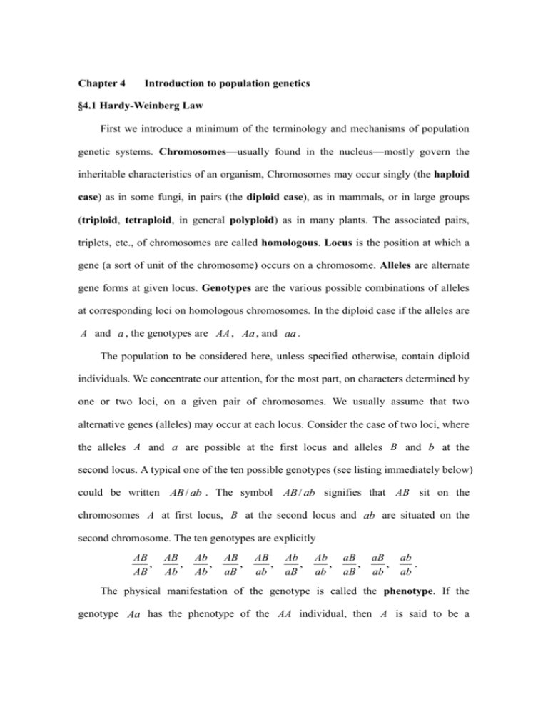
second chromosome. The ten genotypes are explicitly
AB
,
AB
AB
,
Ab
Ab
,
Ab
AB
,
aB
AB
,
ab
Ab
,
aB
Ab
,
ab
aB
,
aB
aB
,
ab
ab
.
ab
The physical manifestation of the genotype is called the phenotype. If the
genotype Aa has the phenotype of the AA individual, then A is said to be a
dominant gene and a is called recessive to A .
We shall assume that an offspring is found by the donation of a gamete (one of
each pair of homologous chromosomes) from each of two parents. In the case of one
locus, each parent, depending on its genotype, may donate either A or a to form a
zygote (fertilized egg) having genotype AA , Aa or aa . Individuals with genotype
AA or aa are homozygotes; Aa is a heterozygote. For two loci, the donated
gametes can be of four kinds, AB , Ab , aB or ab and ten zygotes are possible as
listed previously. Generations are taken to be non-overlapping.
Considering the one locus case, we are primarily interested in tracing the frequencies of
the three genotypes over time. Assume that the population size is very large, effectively
infinite. Let u n , vn , and wn be the frequencies of AA , Aa and aa , respectively,
in the n th generation. In order to follow the vector (u n , vn , wn ) as n increases we
must describe the mating system, i.e., the way mating pairs are to be selected.
One of the most widely studied systems of mating is random-mating. This occurs
when any one individual of one sex is equally likely to mate with any one of the
opposite sex. Thus, in the one locus case above, the mating AA AA would occur with
frequency u n2 at the n th generation. From this mating only AA offspring result.
However, from the mating Aa Aa , AA , Aa and aa offspring will be produced
with probabilities
1
4
,
1
2
,
1
4
respectively. This equally likely case of segregation is
called Mendelian segregation.
In an infinite population, not subject to any outside influences, and in which
random mating takes place the following Hardy-Weinberg Law holds. This states that,
if in a given generation the frequencies of the A and a gene are p and q  1  p
respectively, then in all subsequent generations the frequencies remain the same. We
shall this, and the fact that random mating is equivalent to random union of gametes.
The Hardy-Weinberg Law
We consider a random-mating population which is so large that we may ignore
small chance variations in gene frequencies and treat all processes as being
deterministic. Suppose that at any given locus only two alleles may occur, namely A1
and A2 , and that individuals are diploid but monoecious, (I.e. can act as both male and
female parents). Further, suppose that in any generation, the proportions of the three
genotypes A1 A1 , A1 A2 and A2 A2 are P , 2Q and R respectively.
Since random mating obtains, the frequency of matings of the type A1 A1  A1 A1 is
P 2 , that of A1 A1  A1 A2 is 4 PQ , and so on. We must now consider the outcomes of
each of these matings. If the very small probability of mutation is ignored, elementary
Mendelian rules indicate that the outcome of an A1 A1  A1 A1 mating must be A1 A1 ,
that half the A1 A1  A1 A2 matings will produce A1 A1 offspring, the other half
producing A1 A2 , with similar results for the remaining matings.
It follows that, since A1 A1 offspring can be obtained only from A1 A1  A1 A1
matings (with frequency 1 for such matings), from A1 A1  A1 A2 matings (with
frequency
1
2
for such matings), and from A1 A2  A1 A2 matings (with frequency
1
4
for such matings), and since the frequencies of these matings are P 2 , 4 PQ , 4Q 2 , the
frequency P  of A1 A1 in the following generation is
P   P 2  12 (4 PQ)  14 (4Q 2 )  ( P  Q) 2
(1.1)
2Q   12 (4 PQ)  12 (4Q 2 )  2 PR  12 (4QR )
 2( P  Q)(Q  R),
(1.2)
Similar considerations give
R   14 (4Q 2 )  12 (4QR )  R 2  (Q  R) 2 .
(1.3)
Note that in deriving these results we have assumed no selective differences between
genotypes; that is we have assumed that the genotype of an individual affects neither his
chance of surviving to produce offspring nor the number of such offspring.
The frequencies P  , 2Q  and R  for the next generation are found by replacing
P  , 2Q  and R  by P  , 2Q  and R  and P , 2Q and R by P  , 2Q  and
R  in eqns. (1.1) - (1.3) . Thus, for example,
P   ( P   Q ) 2
 ( P  Q) 2
 P ,
(Using (1.1) and (1.2) )
and similarly it is found that Q   Q  , R   R  . Thus the genotypic frequencies stabled
by the second generation are maintained in the third generation and consequently in all
subsequent generations. Note that frequencies having this property can be characterized
as those satisfying the relation
(Q) 2  PR .
(1.4)
Clearly, if this relation holds in the first generation, so that
Q 2  PR ,
(1.5)
then not only would there be no change in genotypic frequencies between the second
and subsequent generations, but also these frequencies would be the same as those in
the first generation. Populations for which eqn. (1.5) is true are said to have genotypic
frequencies in Hardy-Weinberg form.
Since P  2Q  R  1 , only two of the frequencies P , 2Q and R are
independent. If, further, eqn. (1.5) holds, only one frequency is independent.
Examination of eqns. (1.1) - (1.3) shows that the most convenient quantity for
independent consideration is p  P  Q , that is to say the frequency of the gene A1 .
For convenience the notation q  1  p for the frequency of A2 is often introduced,
but this is not strictly necessary.
The above results may be summarized in the form of a theorem:
Theorem (Hardy-Weinberg). Under the assumptions stated, a population having
genotypic frequencies P (of A1 A1 ), 2Q (of A1 A2 ) and R (of A2 A2 ) achieves
after one generation of random mating, stable genotypic frequencies p 2 , 2 pq , q 2
where p  P  Q and q  Q  R . If the initial frequencies P , 2Q , R are already
of the form p 2 , 2 pq , q 2 , then these frequencies are stable for all generations. This
theorem was established independently by Hardy (1908) and Weinberg (1908).
Random union of gametes
The Hardy-Weinberg law was derived above under a number of simplifying
assumptions, and in order to derive analogous laws under less restrictive assumptions,
and to facilitate the mathematical arguments in general, we will now rederive the law in
a more efficient way.
Any A1 A1 parent will transmit an A1 gene to his offspring. Any such gene is
called, at this stage, a gamete; the union of two gametes forms a zygote or individual.
Now the population considered in Section 1.1 produces A1 gametes with frequency
P  Q and A2 gametes with frequency Q  R ; furthermore, random mating of
individuals is equivalent to random union of gametes. Thus the frequency of A1 A1 in
the following generation is the frequency with which two gametes drawn independently
are both A1 , namely ( P  Q) 2 . This establishes eqn. (1.1) and eqn. (1.2) and (1.3)
follow similarly. The derivation of genotypic frequencies from the argument of random
union of gametes will be used subsequently on a number of occasions.
Dioecious populations
We assumed that individuals are monoecious. While this assumption is of some
independent interest, it was made mainly for convenience; to find how relevant the
derived from it are for other situations, some consideration must be given to populations
where individuals are dioecious.
Suppose that the frequencies of A1 A1 , A1 A2 and A2 A2 among males are PM ,
2QM and RM and among females are PF , 2QF and R F . The gametic outputs from
the two sexes are then PM  QM (of A1 ) and QM  RM (of A2 ) from males and
PF  QF (of A1 ) and QF  RF (of A2 ) from females. The frequencies of he three
genotypes
(in
both
( PM  QM )( PF  QF )
sexes)
,
in
the
following
generation
are
therefore
( PM  QM )(QF  RF )  ( PF  QF )(QM  RM )
,
(QM  RM )(QF  RF ) respectively. The gametic output from this daughter generations
is for both sexes,
1
2
( PM  PF  QM  QF ) (of A1 ) and
1
2
(QM  QF  RM  RF ) (of
A2 ). It is easy to show also that the genotypic frequencies in this following generation
satisfy eqn. (1.5) for both sexes. Thus after one generation of random mating, the
frequencies of three genotypes are the same in both males and females, while a further
generation of random mating ensures that these frequencies are in Hardy-Weinberg
form.
Thus it is reasonable in many circumstances to ignore the dioecious nature of the
population, and we shall indeed almost always do this, mentioning it only on occasions
when special attention is necessary.
Sex-linked genes and multiple alleles
The theory of the preceding section does not apply when the genes in question are
sex-linked, i.e. located on the sex chromosome. To analyse the behaviour for sex-linked
genes, suppose that the male sex is heterogametic and that the initial frequencies are
male
female
A1
A2
A1 A1
A1 A2
A2 A2
pM
qM
PF
2QF
RF
Consideration of the gametic output from each sex shows that in the following
generation these frequencies become
male
A1
A2
PF  QF
QF  RF
female
A1 A1
A1 A2
A2 A2
pM ( PF  QF )
qM ( PF  QF )  pM (QF  RF )
qM (QF  RF ).
The difference between the frequency of A1 in males and the frequency of A1 in
females in the initial generation is
pM  ( PF  QF ) ,
(1.6)
while in the second generation this difference is
PF  QF  { p M ( PF  QF )  12 q M ( PF  QF )  12 p M (QF  RF )}
  12 { p M  ( PF  QF )},
(1.7 )
which in absolute value is half of (1.6) . Clearly, with succeeding generations, this
difference rapidly approaches zero. If, then, it is assumed that initially
pM  PF  QF  p (say), the above theory shows that in one generation the
frequencies
male
female
A1
A2
A1 A1
A1 A2
A2 A2
p
q
p2
2 pq
q2
are attained, and that these frequencies are unaltered in subsequent generations. For
arbitrary initial values of PF and QF , this dose not happen, although a very rapid
convergence to such an equilibrium state occurs. In any event, the important part of the
Hardy-Weinberg law relating to essential stability of genotypic frequencies still stands.
The Hardy-Weinberg law can be extended immediately to the case where more
than two types of genes are allowed at the locus in question. If alleles A1 ,  , Ak
occurs with frequencies p1 ,  , p k , then after one generation of random mating the
2
frequency of Ai Ai is pi , while that of Ai A j ( i  j ) is 2 p i p j ; in subsequent
generations these frequencies are unaltered. The proofs of these statements follow
immediately by considering gamete frequencies, and are omitted; again it is clear that
genotypic frequencies are essentially stable.
Miscellaneous results
Some elementary considerations derived from the Hardy-Weinberg law will be
examined.
In a number of case, the gene A1 is dominant to A2 ; that is, A1 A1 individuals
are indistinguishable from A1 A2 . A common fallacy in such a situation is to suppose
that such dominance ‘spreads’ and that eventually all individuals will be
indistinguishable. Such is not the case, for the stable frequencies derived in Section 1.1
apply irrespective of the existence of dominance; what is gained in the frequency of
dominant individuals by mating of A1 A1 with A2 A2 and of A1 A2 with A2 A2 is
exactly counterbalanced by the loss in frequency through mating of A1 A2 with A1 A2
and of A1 A2 with A2 A2 .
A second consequence of the Hardy-Weinberg law is that if A2 is recessive to A1
and has small frequency, we shall rarely observe recessive individuals. Further, the
parents of recessives will usually both be heterozygotes. For example, if the frequency
q of A2 is 0.001, then the frequency of A2 A2 is 0.000001. The frequency with
which an A2 A2 individual has both parents A1 A2 may be found from the fact that the
parents of an A2 individual must both be  A2 , where the unknown gene is either A1
or A2 . The frequency with which both unknown genes are A1 is (0.999)2=0.998001.
This indicates that the attempted removal of a rare recessive gene by removal of
recessives A2 A2 will have but a minor effect; later on the rate at which such removal
will decrease the frequency of A2 will be considered.
Finally, we remark that the Hardy-Weinberg law has been derived here under the
assumption that generations do not overlap. Thus if this assumption does not hold, the
law itself may not hold. For example, suppose as a continuous time analogue to the
above that in a small time dt a fraction dt of the population dies and is replaced, by
random sampling, from he population at large. Under this system the frequency p of
A1 does not change with time, but if P (t ) is the frequency A1 A1 at time t , then
P(t  dt )  P(t )(1  dt )  p 2 dt .
Passing to the limit in this equation,
dP (t )
  P (t )  p 2 ,
dt
so that
P(t )  {P(0)  p 2 } exp( t )  p 2 .
Clearly a population initially in Hardy-Weinberg equilibrium will remain in equilibrium,
but for non-populations, the equilibrium state is approached asymptotically (and
rapidly). It is clear that the important conclusions derived from the Hardy-Weinberg law
remain unchanged.
The effect of selection
The results given above have been derived under the assumption that no selective
differences exist between the three genotypes A1 A1 , A1 A2 and A2 A2 . In attempting to
discuss the effect of selection one immediately comes up against the problem that
selective values are not properties of genes; they are rather properties of individuals (i.e.
of the whole interacting collection of genes which an individual has), and then refer
properly only to a given environment. Thus it may, and often does, happen that a gene
which is selectively and advantageous against one genetic background is
disadvantageous against another. It will be shown later that such interaction effects can
have major evolutionary consequences, and that it appears difficult even to define a
concept of ‘ independence’ of loci. For the moment, we make the rough approximation
that selective differences depend on the genotype at a given locus; despite the above
remarks, this approximation leads to a number of valuable results.
To be definite, suppose that if, at the time of conception of any generation, the
frequencies of the genotypes are P , 2Q , R , then these genotypes contribute gametes
to
form
the
individuals
of
the
following
generation
in
the
proportions
w11P : 2w12Q : w22 R . (Note that the population is being considered at the time of
formation of zygotes from that gametes of the previous generation. When selective
differences exist, this is the only time when Hardy-Weinberg proportions strictly apply;
later on, when considering finite populations, the population will be counted at the age
of sexual maturity.) The differential reproduction rates may be due to several causes,
including in particular different survival rates and different offspring distributions. The
quantities w11 , w12 , and w22 will be called the ‘fitnesses’ of the three genotypes, and
genotypic frequencies will usually change from one generation to the next.
With the fitnesses given above, the frequencies of the various genotypes in the
following generation now satisfy the equation
P  : 2Q  : R 
 ( w11 P  w12Q) 2 : 2( w11 P  w12Q)( w12Q  w22 R) : ( w12Q  w22 R) 2
 ( p ) 2 : 2 p q  : (q ) 2 ,
(1.8)
where
p  (w11P  w12Q) /( w11P  2w12Q  w22 R).
(1.9)
Clearly, after on generation of random mating, Hardy-Weinberg proportions are
achieved. In the next generation, the same arguments show that
P  : 2Q  : R 
 ( p ) 2 : 2 p q  : (q ) 2
 {w11 ( p ) 2  w12 p q }2 : 2{w11 ( p ) 2  w12 p q }
 {w12 p q   w22 (q ) 2 } : {w12 p q   w22 (q ) 2 }2
(1.10)
It follows that the equation p   p  no longer holds in general. Thus while genotype
frequencies settle down immediately to Hardy-Weinberg form, the more important part
of the Hardy-Weinberg theorem relating to constancy of genotypic frequencies no
longer holds. We shall examine some consequences of this conclusion in the next
section.