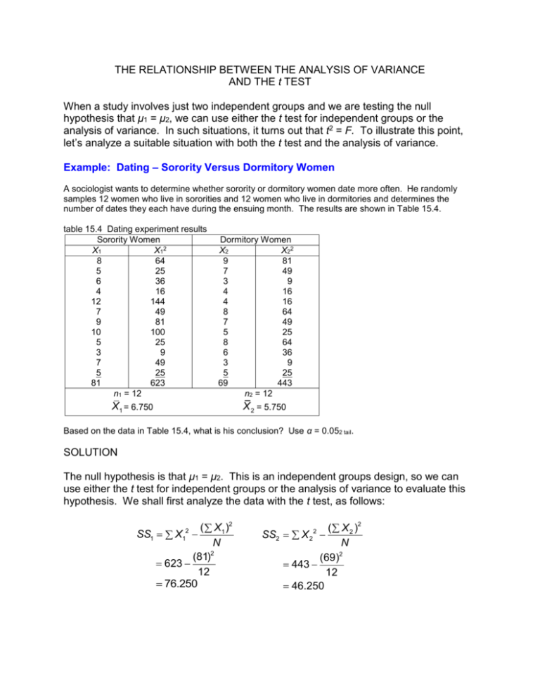
THE RELATIONSHIP BETWEEN THE ANALYSIS OF VARIANCE
AND THE t TEST
When a study involves just two independent groups and we are testing the null
hypothesis that μ1 = μ2, we can use either the t test for independent groups or the
analysis of variance. In such situations, it turns out that t2 = F. To illustrate this point,
let’s analyze a suitable situation with both the t test and the analysis of variance.
Example: Dating – Sorority Versus Dormitory Women
A sociologist wants to determine whether sorority or dormitory women date more often. He randomly
samples 12 women who live in sororities and 12 women who live in dormitories and determines the
number of dates they each have during the ensuing month. The results are shown in Table 15.4.
table 15.4 Dating experiment results
Sorority Women
X1
X12
8
64
5
25
6
36
4
16
12
144
7
49
9
81
10
100
5
25
3
9
7
49
5
25
81
623
n1 = 12
Dormitory Women
X2
X22
9
81
7
49
3
9
4
16
4
16
8
64
7
49
5
25
8
64
6
36
3
9
5
25
69
443
n2 = 12
X 2 = 5.750
X1 = 6.750
Based on the data in Table 15.4, what is his conclusion? Use α = 0.052 tail.
SOLUTION
The null hypothesis is that μ1 = μ2. This is an independent groups design, so we can
use either the t test for independent groups or the analysis of variance to evaluate this
hypothesis. We shall first analyze the data with the t test, as follows:
(  X1 )2
SS1   X 
N
2
(81)
 623 
12
 76.250
2
1
(  X 2 )2
N
2
(69)
 443 
12
 46.250
SS2   X 22 
tobt 

X1  X 2
SS1  SS2
n(n  1)

6.750  5.750
76.250  46.250
12(11)
1.000
 1.038  1.04
0.963
With α = 0.052 tail and df = N – 2 = 22, from Table D in Appendix D,
tcrit = ±2.074
Since ItobtI < 2.074, we retain H0. We cannot conclude that the sorority or dormitory
women date more often.
This problem can also be solved with the analysis of variance. The solution is
shown here.
STEP 1: Calculate SSB:
all
 scores

  X
2


 X2  




n2 
N
2
  X12
SSB  
 n1
 (81)2 (69)2  (150)2



12 
24
 12
 6.000
STEP 2: Calculate SSW:
all
scores
 (  X1 )2 (  X 2 )2 
SSW   X  


n2 
 n1
2
 (81)2 (69)2 
 1066  


12
12 

 122.500
STEP 3: Calculate SST:
all
 scores

  X
all


scores

SST   X 2  
N
2
(150)
 1066 
24
 128.500
2
As a check,
SST  SSB  SSW
128.500  6.000  122.500
128.500  128.500
STEP 4: Calculate df:
dfB  k  1  2  1  1
dfW  N  k  24  2  22
dfT  N  1  24  1  23
STEP 5: Calculate sB2:
sB 2 
SSB 6.000

 6.000
dfB
1
STEP 6: Calculate sW2:
sW 2 
SSW 122.500

 5.568
dfW
22
STEP 7: Calculate Fobt:
Fobt 
sB 2 6.000

 1.078  1.08
sW 2 5.568
With α = 0.05, dfnumerator = 1, and dfdenominator = 22, from Table F,
Fcrit = 4.30
Since Fobt < 4.30, we retain H0. We cannot conclude that sorority or dormitory women
date more often.
Note that we have reached the same conclusion with both the t test and the F test.
A comparison of the two obtained statistics and the associated critical values are shown
here:
tobt2 = Fobt
(1.04)2 = 1.08
1.08 = 1.08
tcrit2 = Fcrit
(2.074)2 = 4.30
4.30 = 4.30
Thus, in the independent groups design, when there are two groups and we are testing
the null hypothesis that μ1 = μ2, tobt2 = Fobt and tcrit2 = Fcrit. Therefore, both tests give the
same result.