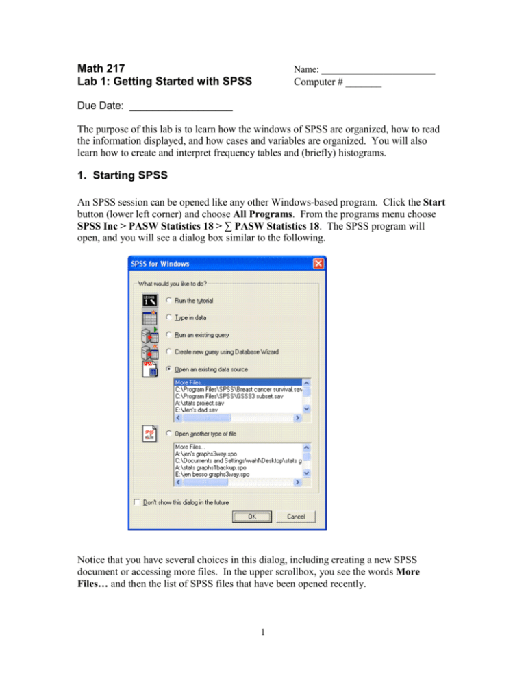
Math 217
Lab 1: Getting Started with SPSS
Name: ________________________
Computer # _______
Due Date: __________________
The purpose of this lab is to learn how the windows of SPSS are organized, how to read
the information displayed, and how cases and variables are organized. You will also
learn how to create and interpret frequency tables and (briefly) histograms.
1. Starting SPSS
An SPSS session can be opened like any other Windows-based program. Click the Start
button (lower left corner) and choose All Programs. From the programs menu choose
SPSS Inc > PASW Statistics 18 > ∑ PASW Statistics 18. The SPSS program will
open, and you will see a dialog box similar to the following.
Notice that you have several choices in this dialog, including creating a new SPSS
document or accessing more files. In the upper scrollbox, you see the words More
Files… and then the list of SPSS files that have been opened recently.
1
The file you need to open for Lab 1 is located at the following address:
C:\Program Files\SPSSInc\PASWStatistics 18\Samples\English\GSS93 subset.sav.
If the file you need is not shown in the upper scrollbox, select More Files… by selecting
it and then clicking OK. You get a dialog box similar to the one shown below.
You can use the Open Data dialog to locate and open the file GSS93 subset.sav (see
pathname, given above). Once you’ve opened the data file, you should see the following:
2
Every time you open an SPSS data file, you get what is called a Data Editor window. It
can appear in one of two views: a Data View and a Variable View. At the bottom left
of the window are tabs that allow you to display one or the other of the two views. Try
clicking on Variable View; you should obtain a window like the one shown below.
In this view, each row contains the information pertaining to one variable. We will learn
more about this variable information after we take a look at the other view, the Data
View.
When you click on the Data View tab of the SPSS Data Editor, you see the data itself,
and you can modify it directly in this window (similar to an Excel spreadsheet). Perform
the operations indicated below and observe their effects on the screen.
1. Display the Value Labels instead of the codes by selecting Value Labels under
View. Toggle back and forth between labels on and labels off to see the effect.
2. Read the label of any variable by lingering with the mouse on any column
heading.
3. Enlarge any column by positioning the mouse on the edge separating the column
headings, and drag to the right.
4. Select Variables under the Utilities menu to see the dialog box shown below.
Scroll down the list of variables. To see the details of a variable, highlight that
variable name in the list of variables.
3
Notice the following information in the right side of the window:





The variable label, which explains what the variable measures.
The variable type. This is the format of the numerical values or labels you enter.
For example, F1 means that the format used for that variable is one space long,
with no decimals. F5.2 means that 5 spaces are reserved to write the values of
that variable, of which 2 are decimals (like 123.45).
The missing values. For each variable, some of the answers should not be taken
into account in the statistics, such as when somebody refuses to answer, or when
the question does not apply to that person. We give codes for the values ‘Refuses
to answer’ and ‘Does Not Apply’, but we must indicate that these answers are not
to be treated like the other answers. We label them “missing values.”
The measurement level. In this data file, for example, the variable marital status
has been defined to be ordinal, meaning it is a categorical variable whose
categories have a natural ordering. Categorical variables with no reasonable
ordering for their categories should use nominal measurement. Quantitative
variables, like age, should use scale measurement.
A list of value labels (if any), and their corresponding codes. Value labels
describe the different categories which are possible for a categorical variable, and
can describe missing values for any type of variable.
4
Here is your assignment:
 Read the beginning of the SPSS online tutorial. Go to Help > Tutorial.
 Starting from the introduction, read the tutorial. STOP when you reach Creating
Charts, and close the tutorial.
 Go back to the GSS93 subset Data Editor window.
 Use the Analyze > Descriptive Statistics > Frequencies dialog to create
appropriate frequency tables and answer the following questions about the
subjects in the GSS93 subset data file. (Start by figuring out the relevant variable
names.)
1. What percentage of the respondents are male? _______ Female? _______
2. Find an age so that half the sample are younger or equal to that age, the other half
being older: ______ This age is called the ___________ .
3. What percentage of the respondents (of those who answered "legal" or "not legal"
-- see valid percentage) believe marijuana should be made legal? ________
4. What percentage of the respondents (use valid percentage) believe that humans
definitely did not evolve from animals? ________
5. What proportion of respondents have a "valid" (not a "missing") response to the
question about their age when they were first married? _________
6. Which numerical codes indicate "missing" values for the "age when first married"
variable? _____________ What are the reasons for these missing answers
(explain briefly)?
7. Only a scale (quantitative) variable can be used to generate a histogram. Almost
all the variables in GSS93 subset have been designated as ordinal variables, many
of them erroneously. Fix the measurement level for the "age when first married"
variable as follows, and make a histogram:
a) Go to Variable View.
b) Locate the variable agewed. Change it from ordinal to scale measurement,
then go back to Data View.
c) From the Graphs menu choose Legacy Dialogs > Histogram. Drag age
when first married to the empty rectangle labeled "variable."
d) Use the Titles button to title your graph, "Distribution of Respondent Age
When First Married" and click Continue.
e) Click OK to draw the histogram. It should appear at the bottom of the output
viewer.
f) On the following page, write a brief paragraph describing the distribution of
the agewed variable in the GSS93 dataset. Include sentences regarding the
overall shape (how many major peaks? symmetrical? skewed?), center
5
(median valid response), spread (minimum and maximum values), location of
peak(s), and discussion of any outliers (do any respondents have highly
unusual marriage ages compared to other respondents?). Note that the
frequency table you made for this variable will be helpful in answering some
of these questions.
Write your paragraph here:
 Go back to the desktop. In the My Documents folder on your computer, create a
new folder labeled with your name.
 Back in the output viewer window of SPSS, use File > Save As ... to save a copy
of your SPSS output file to the folder you created. The output file should contain
all your frequency tables and the agewed histogram. Name your output file
Lab 1 so you can distinguish it from future labs.
 DO NOT save the GSS93 subset.sav data file.
 Your folder inside My Documents is a good place to save copies of all your SPSS
work this term. Any files which are very important should also be saved to your
portable memory device or sent to your email account.
 Make a habit of using the same computer as much as possible throughout the
term.
6