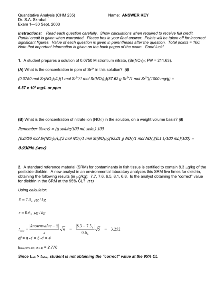
Quantitative Analysis (CHM 235)
Dr. S.A. Skrabal
Exam 1—30 Sept. 2003
Name: ANSWER KEY
Instructions: Read each question carefully. Show calculations when required to receive full credit.
Partial credit is given when warranted. Please box in your final answer. Points will be taken off for incorrect
significant figures. Value of each question is given in parentheses after the question. Total points = 100.
Note that important information is given on the back pages of the exam. Good luck!
1. A student prepares a solution of 0.0750 M strontium nitrate, (Sr(NO3)2; FW = 211.63).
(A) What is the concentration in ppm of Sr2+ in this solution? (8)
(0.0750 mol Sr(NO3)2/L)(1 mol Sr2+/1 mol Sr(NO3)2)(87.62 g Sr2+/1 mol Sr2+)(1000 mg/g) =
6.57 x 103 mg/L or ppm
(B) What is the concentration of nitrate ion (NO3-) in the solution, on a weight:volume basis? (8)
Remember %w:v) = (g solute/100 mL soln.) 100
(0.0750 mol Sr(NO3)2/L)(2 mol NO3-/1 mol Sr(NO3)2)(62.01 g NO3-/1 mol NO3-)(0.1 L/100 mL)(100) =
0.930% (w:v)
2. A standard reference material (SRM) for contaminants in fish tissue is certified to contain 8.3 g/kg of the
pesticide dieldrin. A new analyst in an environmental laboratory analyzes this SRM five times for dieldrin,
obtaining the following results (in g/kg): 7.7, 7.6, 6.5, 8.1, 6.8. Is the analyst obtaining the “correct” value
for dieldrin in the SRM at the 95% CL? (11)
Using calculator:
x  7.3 4 g / kg
s  0.6 6 g / kg
t calc 
known value  x
s
n

8.3  7.3 4
0.6 6
5
 3.252
df = n -1 = 5 -1 = 4
ttable(95% CL; df = 4) = 2.776
Since tcalc > ttable, student is not obtaining the “correct” value at the 95% CL
3. A pharmaceutical quality control lab performed analyses for morphine in 60 mg tablets. The results of
eight analyses yielded the following results (in milligrams): 58.4, 59.3, 54.2, 58.5, 59.1, 60.0, 57.8, 58.3.
(A) Should any of the results be rejected by the Q-test at the 90% CL? (6)
54.2 , 57.8, 58.3, 58.4, 58.5, 59.1, 59.3, 60.0
54.2 is the questionable point:
Q = gap/range = (57.8 – 54.2) / (60.0 – 54.2) = 3.6 / 5.8 = 0.621
Qtable(90% CL; n = 8) = 0.468
Since Qcalc > Qtable, point can be rejected at the 90% CL
(B) Report the mean, standard deviation, and relative standard deviation of the acceptable analyses. (10)
Using calculator, the statistics for the 7 remaining data points are:
x  58.7 7 mg or 58.8 mg
s  0.7 3 mg or 0.7 mg
 0.7 3 mg 
100  1.2 % or 1%
rsd  
58
.
7
mg
7


4. What is the percent relative uncertainty in a measurement of 0.523 mL of H2O in a 2.000 mL buret if the
absolute uncertainty of the buret is  0.002 mL? (10)
 0.002 mL 
 absolute uncert . 
100  0.38 % or 0.4%
% relative uncert.  
100  
 measurement 
 0.523 mL 
2
5. The concentration of ethanol in a Portuguese wine has been analyzed using two different methods.
Using method 1, seven analyses yielded a concentration of 2.653  0.082 M. Five analyses using method 2
yielded a concentration of 2.42  0.15 M. The uncertainties are standard deviations.
(A) Use the F-test (95% CL) to verify that there is no difference between the standard deviations of the two
methods. (7)
Fcalc 
s12
where s1  s 2
s 22
Fcalc 
(0.15 ) 2
 3.35
(0.08 2 ) 2
df = 5 -1 = 4 for s1 data; df = 7 -1 = 6 for s2 data
Ftable(95% CL, df = 4,6) = 4.53
Since Fcalc < Ftable, standard deviations of the two data sets are not significantly different at the 95%
CL
(B) Determine whether or not the means of the two methods are the same at the 95% CL. (12)
Use t-test for the comparison of means:
s pooled 
t calc 
s12 (n1 1)  s 22 (n2 1)
n1  n2  2

x1  x 2
n1 n2
s pooled
n1  n2

2.65 3  2.4 2
0.1142

(0.08 2 ) 2 (7 1)  (0.15 ) 2 (5 1)
7  5 2
(7)(5)
75
 0.1142
 3.484
df = 7 + 5 – 2 = 10
ttable(95% CL, df = 10) = 2.228
Since tcalc > ttable, means of the two methods are significantly different at the 95% CL
6. A testing laboratory determined the total dissolved phosphate concentration in 90 samples of a brand of
liquid detergent. The results obtained were 25.84  0.97 mg/g, where the uncertainty is a standard
deviation. (Note that I am keeping one more significant digit for the mean and standard deviation for this
exercise). Calculate the 50% and 99% confidence intervals for these data. Express the confidence
intervals to two decimal places. (10)
50% CI: ttable(50% CL, df = 89) = 0.678 (by interpolation)
x
ts
n
 25.84 
(0.678)(0.97)
90
 25.84  0.06 9 mg / g
99% CI: ttable(99% CL, df = 89) = 2.638 (by interpolation)
x
ts
n
 25.84 
(2.638)(0.97)
90
 25.84  0.27 mg / g
3
7. A calibration curve for dissolved silicate was obtained by measuring absorbances in a
spectrophotometric analysis, using Si standards in a range from 0 to 7.5 μM. The data were analyzed using
the LINEST function in Excel®, and the following unedited parameters of the regression were calculated:
slope: 0.057771 ± 0.0005352
y-intercept: 0.001296 ± 0.000593
std. dev. of y values: 0.001145
An unknown sample was analyzed, yielding an absorbance of 0.142. The blank was found to be 0.001.
(A) Write the linear regression equation for this analysis, including the uncertainties, using the correct
number of significant figures. (6)
y ( sy) = m ( sm)  x ( sx) + b ( sb)
y ( 0.0011) = 0.05777 ( 0.00053)  x ( sx) + 0.00129 ( 0.00059)
(B) Determine the silicate concentration and its absolute and relative uncertainty in the unknown. (12)
Rearrange equation above to solve for x ( sx)
Blank-corrected absorbance (signal) = 0.142 – 0.001 = 0.141
x ( s x ) 
y ( s y )  b ( sb )

m ( s m )
x  (s x )  2.418  s x M
Now determine sx (relative and absolute) and round the answer correctly
enum  (0.0011 ) 2  (0.00059 ) 2
%enum 
0.141( 0.0011 )  0.0012 9 ( 0.00059 )
0.0577 7 ( 0.00053 )
 0.0012
0.0012
(100)  0.8 5 %
(0.141  0.0012 9 )
%edenom 
0.00053
(100)  0.91%
0.0577 7
%eoverall  (0.85 %) 2  (0.91%) 2  1.2 %
(1.2%)(2.418 M) = (0.012)(2.418 M) = 0.029 M
2.418  0.029 M or 2.42  0.03 M
Relative uncertainty: 1.2 or 1%
4
Useful information
Standard deviation: s 
 ( xi  x ) 2
i
n 1
Confidence interval:   x 
ts
n
where degrees of freedom = n – 1.
Comparison of means (when standard deviations are not significantly different):
t calc 
x1  x 2
n1 n2
s pooled
n1  n2
s pooled 
s12 (n1 1)  s 22 (n2 1)
n1  n2  2
where degrees of freedom = n1 + n2 - 2
Comparing measured result to known result:
t calc 
known value  x
s
n
where degrees of freedom = n – 1.
Fcalc
s12
 2
s2
where s1 > s2 and degrees of freedom is n1 – 1 and n2 -1
en  e12  e22  e32  ...  en21
%en  %e12  %e22  %e32  ...  %en21
y = mx + b
Q = gap/range
5