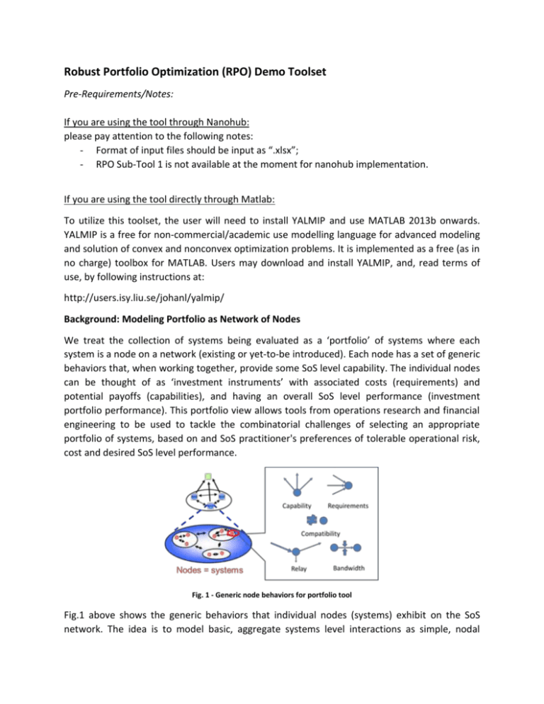
Robust Portfolio Optimization (RPO) Demo Toolset
Pre-Requirements/Notes:
If you are using the tool through Nanohub:
please pay attention to the following notes:
- Format of input files should be input as “.xlsx”;
- RPO Sub-Tool 1 is not available at the moment for nanohub implementation.
If you are using the tool directly through Matlab:
To utilize this toolset, the user will need to install YALMIP and use MATLAB 2013b onwards.
YALMIP is a free for non-commercial/academic use modelling language for advanced modeling
and solution of convex and nonconvex optimization problems. It is implemented as a free (as in
no charge) toolbox for MATLAB. Users may download and install YALMIP, and, read terms of
use, by following instructions at:
http://users.isy.liu.se/johanl/yalmip/
Background: Modeling Portfolio as Network of Nodes
We treat the collection of systems being evaluated as a ‘portfolio’ of systems where each
system is a node on a network (existing or yet-to-be introduced). Each node has a set of generic
behaviors that, when working together, provide some SoS level capability. The individual nodes
can be thought of as ‘investment instruments’ with associated costs (requirements) and
potential payoffs (capabilities), and having an overall SoS level performance (investment
portfolio performance). This portfolio view allows tools from operations research and financial
engineering to be used to tackle the combinatorial challenges of selecting an appropriate
portfolio of systems, based on and SoS practitioner's preferences of tolerable operational risk,
cost and desired SoS level performance.
Fig. 1 - Generic node behaviors for portfolio tool
Fig.1 above shows the generic behaviors that individual nodes (systems) exhibit on the SoS
network. The idea is to model basic, aggregate systems level interactions as simple, nodal
behaviors that are applicable to a wide variety of inter-system connections. Fig.1 shows the five
most intuitive nodal interactions where:
•
Capability: Nodes have finite supply of capabilities that are limited by quantity and
number of connections.
•
Requirements: Nodes have requirements to enable inherent capabilities. Requirements
are fulfilled by receiving connections from other nodes that possess a capability to fulfill said
requirements.
•
Relay: Nodes can have the ability to relay capabilities between adjacent nodes. This can
include excess input of capabilities that are used to fulfill node requirements.
•
Bandwidth: Total amount of capabilities or number of connections between nodes are
bounded by connection bandwidth.
•
Compatibility: Nodes can only connect to other compatible nodes.
The performance of a SoS is related to the ability of the connected network of individual
systems to fulfill SoS level objectives. It is assumed that these core objectives can be at least,
approximated quantitatively. We describe 3 versions of the RPO tool (here, termed ‘sub-tools’
in the next section) that will be used, following the above logic of modeling the portfolio as a
network of nodes, to perform SoS Architectural Analysis.
Description of RPO Tools
This section briefly illustrates tool features for the RPO toolset. There are three sub-tools
available within the RPO toolset – each sub-tool solves a different focus of the robust portfolio
optimization option.
A brief description of each RPO sub-tool is given here:
RPO Sub-Tool 1: Robust Portfolio: Capability vs. Uncertain Development
Solves the robust optimization problem of selecting different ‘portfolios’ of systems where the
payoffs come from the collective capabilities of the optimized portfolio; this ‘payoff’ from
capabilities is balanced against the risks in estimated development and integration time(s) of
systems. Formulation of this tool includes consideration for robustness against uncertainty in
the estimated distributions of development (and integration) times.
RPO Sub-Tool 2– Robust Operational Constraints (Bertsimas-Sim)
Solves the portfolio problem but with robustness control on individual linear constraints.
Method uses Bertsimas-Sim formulation that assumes symmetric uncertainty for numerical
value of capabilities of nodes.
RPO Sub-Tool 3 – Robust Operations using Conditional Value-at-Risk (CVaR)
Solves a robust portfolio optimization problem where the capabilities (payoff) of nodes that
contribute to the overall SoS performance, uses simulation data. Outcomes of capability from
each node are a simulated set of values and results are used to mitigate downside risks.
Formulation is based on Conditional Value-at-Risk (CVaR) measure used in financial
engineering.
General Description of Input File
Inputs to the method come from an input file labelled “InputData.xlsx”. The first three
worksheets of the Excel file are used to generate the relevant optimization problem for the
Naval Warfare Scenario (NWS) demonstration problem.
Data File Inputs
Sheet 1 – Main Data File
No.
1
2
3
4
5
6
7
8
9
10
11
12
13
14
15
16
17
18
19
20
21
22
23
System Name
GroundSystem 1
GroundSystem 2
GroundSystem 3
GroundSystem 4
GroundSystem 5
Satellite System 1
Satellite System 2
Satellite System 3
Satellite System 4
Satellite System 5
UAV-1
UAV-2
Manned Aircraft 1
Manned Aircraft 2
Manned Aircraft 3
Ship-1
Ship-2
Ship-3
Power System 1
Power System 2
Power System 3
Power System 4
Power System 5
Capabilities (Outputs)
Requirements (Inputs)
SoS CAP 1 SoS CAP 2 SoS CAP 3 Power. Comm. Req 1 Req 2 Req 3 Reg 4 Req 5
0
0
0
150
0
0
0
0
0
0
0
0
0
300
0
0
0
0
0
0
0
0
0
450
0
0
0
0
0
0
0
0
0
600
0
0
0
0
0
0
0
0
0
750
0
0
0
0
0
0
0
0
100
0
0
75
95
0
0
0
0
0
200
0
0
125
150
0
0
0
0
0
300
0
0
150
250
0
0
0
0
0
400
0
0
175
350
0
0
0
0
0
500
0
0
185
450
0
0
0
20
0
0
0
0
100
0
0
0
0
30
0
0
0
0
200
0
0
0
0
40
0
0
0
0
300
0
0
0
0
50
0
0
0
0
120
0
0
0
0
60
0
0
0
0
300
0
0
0
0
0
5
0
0
0
50
0
0
0
0
0
10
0
0
0
150
0
0
0
0
0
20
0
0
0
200
0
0
0
0
0
0
0
0
100
0
0
0
0
0
0
0
0
0
200
0
0
0
0
0
0
0
0
0
300
0
0
0
0
0
0
0
0
0
400
0
0
0
0
0
0
0
0
0
500
0
0
0
0
0
Cost
[$]
10000
20000
300000
400000
500000
500000
650000
750000
850000
900000
200000
300000
400000
450000
500000
500000
600000
700000
50000
60000
70000
80000
90000
CAP 1
0
0
0
0
0
0
0
0
0
0
0
0
0
0
0
0
0
0
0
0
0
0
0
Uncertain. Capabilities (+/- delta)
CAP 2
CAP 3
CAP 4
CAP 5
0
0
30
0
0
0
60
0
0
0
150
0
0
0
300
0
0
0
500
0
0
0
32
0
0
0
12
0
0
0
14.6
0
0
0
8.4
0
0
0
49
0
0
0
30
0
0
0
10.5
0
0
0
10.9
0
0
0
10.3
0
0
0
13.4
0
0
0
25
0
0
0
35
0
0
0
50
0
0
0
0
10
0
0
0
20
0
0
0
40
0
0
0
80
0
0
0
150
Columns 1-3 (SoS Level Capabilities)
These columns denote capabilities provided by each listed node towards an SoS-level objective
(for example, in a missile defense related SoS scenario, this may relate to a missile range). An
entry of zero means that the listed system does not provide the capability listed in the
corresponding column.
Columns 4-5 (Node Level Capabilities)
These columns denote capabilities provided by each listed node towards general nodal
objective (for example, in a missile defense related SoS scenario, some nodes may provide a
power and/or communication bandwidth to the SoS level nodes that have a missile capability.
Num
Links
1
1
1
1
1
1
1
1
1
1
1
1
1
1
1
1
1
1
1
1
1
1
1
An entry of zero means that the listed system does not provide the capability listed in the
corresponding column.
Columns (6-7) (Node Level Requirements)
These columns denote requirements for each listed system. For example, systems that have a
missile range capability may have requirements on amount of power needed or total
communications bandwidth needed to operate.
Columns (8-10, 12-14) Inactive
(These columns are inactive for the demo but will be used to facilitate future requirements
abilities in the workbench.)
Column 11 – Cost of each system
Lists cost (here, monetary but can be any cost in general) for each system.
Column 15-16 – Uncertainties
Here, the uncertainties in each corresponding capability is listed. The columns of 15-16
correspond to uncertainties for the numbers in columns 4 and 5 respectively, denoting
uncertainties in power and communications capabilities in each node.
Sheet 2 – System Compatibilities and Option Selection
Here, the table on the left lists compatibilities between systems listed in the main file by the
user. For example, in this provided sheet, since system 1 and system 2 cannot be selected –
there is an entry that system 1 has ‘2’ under incompatibilities. Up to 5 systems can be input as
being incompatible. Also, there is not a need for duplicative declaration of the same constraint
for system 2 – meaning, that under the system 2 row, the user does not need to re-declare that
system 2 is incompatible with system 1.
The table on the right labelled ‘Can have Options’ allows the user to select range limits based
on inequality constraints. For example, the first row in the table indicates that only one system,
from the list of systems 1 to 5, can be selected. The second row indicates that up to two
systems
can
be
selected
from
the
list
of
systems
6
to
10.
The table labelled “must select options” allows the user to select limits based on equality
constraints. For example, in this table, the user must select one system from the list of systems
ranging from systems 16 to 18.
Sheet 3 – Must have systems
System
1
2
3
4
5
6
7
8
9
10
11
12
13
14
15
16
17
18
19
20
21
22
23
(1=Yes, 0 = No)
0
0
0
0
0
0
0
0
0
0
0
0
0
0
0
0
0
0
0
0
0
0
0
In this sheet, the user defines which specific systems must already be in the list of systems
selected – this is useful for defining existing systems that must already be part of the
architectures being explored. Note that this is different from the prior table description on
‘Must Select Options’ in that the declaration of selecting a system must be for specific systems.
Sheet 4 – Must have links (Inactive in this version for now)
In this sheet, declarations for various ‘must have’ connections between systems, for each type
of available capability attribute. (We deactivate this in this version of the toolset for simplicity)
Sheet 5 – Development Covariance
In this sheet, the user can define the estimated variances in development time and integration
time for each system in the list. The diagonal terms of the matrix (Mij) refer to the variance in
development time The off-diagonal terms refer to the time it takes for system (i) to be
integrated with system (j). For example, we refer to the following table snippet of Sheet 5
below:
System
1
2
3
4
5
1
0.78
0.49
0.40
0.30
0.47
2
0.49
0.93
0.28
0.54
0.38
3
0.40
0.28
0.62
0.50
0.31
4
0.30
0.54
0.50
0.68
0.34
5
0.47
0.38
0.31
0.34
1.14
6
0.40
0.61
0.46
0.64
0.47
7
0.23
0.29
0.51
0.52
0.60
Here, the M11 term takes a value of 0.78 and is the variance in time (say months) for system 1
to be developed. M12 takes a value of 0.49 and is the variance in the time it takes for system 1
and system 2 to be integrated. Notice that M21 also takes the same value as this is due to the
assumption that the time to integrate system 2 and system 1 is the same vice versa of course.
(Data in this sheet is used specifically in RPO Sub-tool 1)
Sheet 6 – Simulated Capabilities
In this sheet, the user can define the simulated outcomes of capabilities for each node in the
system, if available. Simulated outcomes are recorded as vectors where each column is the
simulated outcome for each system following some experiment/simulation.
SoS Workbench Demonstration Walk Through
In this section, we step through the demonstrative version of the workbench that utilizes each
of the sub-tools within the RPO toolset. Steps 1 – XX are common to all three sub-tools and will
involve loading the data, choosing a method (depending on analysis that needs to be
performed) and
Step 1 – Upon clicking the robust portfolio toolset from the main graphical user interface (GUI),
the user will be presented with the following main screen of the RPO demo toolset.
The user can input the name of the provided Excel file that contains prior loaded information
(filename is “InputData.xls” as shown below). (InputData.xls will contain some demonstration
data) (Note: if you are using the tool through Nanohub, please input “InputData.xlsx”; same
for all the following files)
The user should wait until the data is loaded into the GUI (takes about a minute). The data from
the Excel spreadsheet will be shown within the GUI as the following:
Step 2 – The user can then select the relevant method for analysis, based on the data input into
the Excel spreadsheet. Select the appropriate method, based on desired analysis.
**Special Menu: RPO Sub-Tool 2– Robust Operational Constraints (Bertsimas-Sim)
If selecting the Bertsimas-Sim method, note that there are 2 options for analysis; the ability to
look at 1 or 2 robust constraints simultaneously. These correspond to Columns Q and R in the
the worksheet labelled “Main Sheet” of the input excel file : InputData.xls(here, for the demo,
we restrict to two constraints of power requirements being satisfied, and power and
communications simultaneously)
The user then clicks on ‘Generate Portfolios’ to generate the relevant tradespace that utilizes
the robust optimization methodology. A “waitbar” will appear that displays the progress of the
optimizations.
The following image snapshot results consequently for each of the Sub-Tools in the toolset
when the demo input xls file is run:
Here we will show usage of the tool with the Bertsimas-Sim Sub-Tool – instructions translate
similarly for other tools.
The above image shows two graphs on the right (here, in this case, the Bertsimas-Sim subtool
based analysis). The top graph shows the SoS level performance index against level of
robustness in the Communications layer of the overall selected portfolio of systems. Each point
on the graph is a collection of systems put together that result in the corresponding level of
performance and robustness. The bottom graph shows associated cost of corresponding points
on the top graph’s frontier.
Step 3 – If a user wishes to interrogate a particular solution point, the user may click on the
following button, and select a point on the top graph. (A blinking indicator sign will activate)
Upon selecting a point, the following screen snapshot illustrates the displayed information.
Note that as a result of clicking a specific point on the top graph, the GUI will display the
solution at that point of the frontier and list the systems that, when selected to operate
together, will result in the indicated SoS performance on the graph. Additionally, the user can
display topological information of the chosen architecture point on the graph by selecting the
“View topology” button.
The topology of the architecture, based on listed constraints (here, power and communications
constraints) are subsequently shown:
Step 4 – User can repeat analysis for multiple dimension case of ‘Power and Communications’
to see the tradeoffs in robustness by simultaneously considering the power and
communications requirements being met.
The user can repeat the analysis for multi-dimensions (here, selection of power and
communications layer allows for robustness of both constraints to be viewed as a surface plot.
Current version does not permit interrogation of points on the surface (will be included under
future RT-134 version).
Future updates: This version of the portfolio tool within the SoS Analytic Workbench is
currently being developed further through a new research task of RT-134. Extensive updates to
this demonstrative version will be done, and, will include additional features to accommodate
further inputs from the user as well.
README Button: Displays disclaimer information on software use and utilization of YALMIP
toolbox as part of RPO toolset. Please read information by clicking on button.