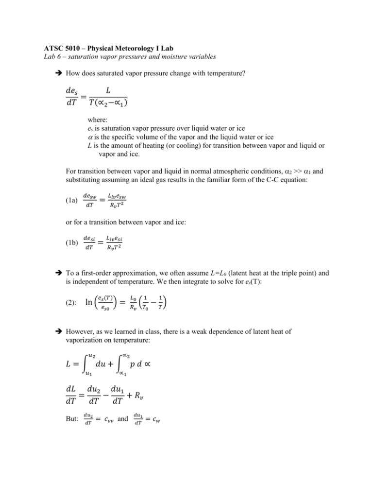
ATSC 5010 – Physical Meteorology I Lab
Lab 6 – saturation vapor pressures and moisture variables
 How does saturated vapor pressure change with temperature?
𝑑𝑒𝑠
𝐿
=
𝑑𝑇 𝑇(∝2 −∝1 )
where:
es is saturation vapor pressure over liquid water or ice
is the specific volume of the vapor and the liquid water or ice
L is the amount of heating (or cooling) for transition between vapor and liquid or
vapor and ice.
For transition between vapor and liquid in normal atmospheric conditions, 2 >> 1 and
substituting assuming an ideal gas results in the familiar form of the C-C equation:
(1a)
𝑑𝑒𝑠𝑤
=
𝑑𝑇
𝐿𝑙𝑣 𝑒𝑠𝑤
𝑅𝑣 𝑇 2
or for a transition between vapor and ice:
(1b)
𝑑𝑒𝑠𝑖
=
𝑑𝑇
𝐿𝑖𝑣 𝑒𝑠𝑖
𝑅𝑣 𝑇 2
 To a first-order approximation, we often assume L=L0 (latent heat at the triple point) and
is independent of temperature. We then integrate to solve for es(T):
(2):
𝑒𝑠 (𝑇)
ln (
𝑒𝑠0
)=
𝐿0
𝑅𝑣
1
1
(𝑇 − 𝑇)
0
 However, as we learned in class, there is a weak dependence of latent heat of
vaporization on temperature:
𝑢2
∝2
𝐿 = ∫ 𝑑𝑢 + ∫ 𝑝 𝑑 ∝
𝑢1
∝1
𝑑𝐿 𝑑𝑢2 𝑑𝑢1
=
−
+ 𝑅𝑣
𝑑𝑇
𝑑𝑇
𝑑𝑇
But:
𝑑𝑢2
𝑑𝑇
= 𝑐𝑣𝑣 and
𝑑𝑢1
𝑑𝑇
= 𝑐𝑤
where cw is specific heat capacity of liquid (for phase transition between vapor and ice we
would consider ci). Thus:
𝑑𝐿
= 𝑐𝑣𝑣 − 𝑐𝑤 + 𝑅𝑣 = 𝑐𝑝𝑣 − 𝑐𝑤
𝑑𝑇
Integrating from some known state, L0 and T0:
(3a): 𝐿𝑙𝑣 (𝑇) = 𝐿0 − (𝑐𝑤 − 𝑐𝑝𝑣 )(𝑇 − 𝑇0 )
(3b): 𝐿𝑖𝑣 (𝑇) = 𝐿0 − (𝑐𝑖 − 𝑐𝑝𝑣 )(𝑇 − 𝑇0 )
Equations 3 (a & b) work pretty well, but we are still ignoring the (slight) dependence of
specific heat capacity on temperature. Ugh…… So, we are going to breakdown and
consider an empirical function for es on temperature. Here we are ignoring the solution to
C-C and computing directly esw (and esi) as a function of temperature.
For saturation vapor pressure over liquid:
0.58002206 ∗ 104
𝐿𝑂𝐺(𝑒𝑠𝑤 ) = −
+ 0.13914993 ∗ 101 − (0.48640239 ∗ 10−1 )𝑇
𝑇
+ (0.41764768 ∗ 10−4 )𝑇 2 − (0.14452093 ∗ 10−7 )𝑇 3
+ (0.65459673 ∗ 101 ) ∗ 𝐿𝑂𝐺(𝑇)
For saturation vapor pressure over ice:
0.56745359 ∗ 104
𝐿𝑂𝐺(𝑒𝑠𝑖 ) = −
+ 0.6392527 ∗ 101 − (0.96778430 ∗ 10−2 )𝑇
𝑇
+ (0.62215701 ∗ 10−6 )𝑇 2 + (0.20747825 ∗ 10−8 )𝑇 3 − (0.94840240
∗ 10−12 )𝑇 4 + (0.41635019 ∗ 101 ) ∗ 𝐿𝑂𝐺(𝑇)
Exercise:
Assume L0 = 2.500×106 J/kg at 0 C
Assume es0 = 611.21 Pa at 0 C
1. Assuming no variation of L on temperature, solve (2) for esw(T) and for esi(T)
2. From the functional relationship in equation (3), substitute into the Clausius-Clapeyron
equation and integrate. You will have a new, more complicated expression for es(T).
3. Build a function called sat_vapor that takes an input of temperature (vector) in Kelvin
and returns a corresponding vector of saturation vapor pressures in Pascal. Allow your
function to have keywords: ice, liquid, Lconst, Lfunction, polynomial. Upon calling
sat_vapor, if keyword ‘ice’ is set, the saturation vapor pressure over ice is computed;
likewise if keyword ‘liquid’ is set, the saturation vapor pressure over liquid is computed.
If keyword ‘Lconst’ is set use the approximation that L is constant over the temperature
range to compute saturation vapor pressure. If keyword ‘Lfunction’ is set use the
functional relationship given in equations 3 (a & b) for latent heats to compute saturation
vapor pressure. If keyword ‘polynomial’ is set, use the polynomial fit to compute directly
the saturation vapor pressure.
4. Build a procedure (atsc5010_yourname_lab6) that produces a vector of temperatures
from -40 to +100 C with 0.1 C resolution. In this procedure:
a. Call sat_vapor several times, each time with the appropriate keyword(s) set to
compute saturation vapor pressure over ice and/or over liquid for the temperature
range from -40 to +100 C.
b. Plot a graph (P-T diagram) showing the saturation vapor pressure over liquid and
ice from -40 C to 100 C. Use red for ‘Lconstant’, blue for ‘Lfunction’, and black
for ‘polynomial’. For saturation vapor pressure over liquid at temperatures below
0 C, use a dashed line. All other lines should be solid.
c. Consider the comparison between ‘Lconstant’ and ‘polynomial’. For both
saturation vapor pressure over liquid, plot the difference between the computed
values using ‘Lconstant’ and ‘polynomial’ as a function of temperature. Do the
same for saturation vapor pressure over ice.
d. Similar to (c), Plot the percent difference between the two computations as a
function of temperature (both for saturation vapor pressure over liquid and
saturation vapor pressure over ice).
e. Similar to (c) and (d), construct similar plots comparing the computations
between ‘Lfunction’ and ‘polynomial_fit’.
f. Now consider our most accurate model, ‘polynomial’, only. Noting that relative
humidity wrt liquid, h, is defined as e/esw and relative humidity wrt ice, hi, is
defined as e/esi. Consider a cloud that is composed of liquid water and ice crystals
(mixed phase cloud). If the cloud is just saturated wrt to liquid, calculate (and
plot) the relative humidity wrt ice as a function of temperature.
Remember to use axis labels and titles on all your plots.