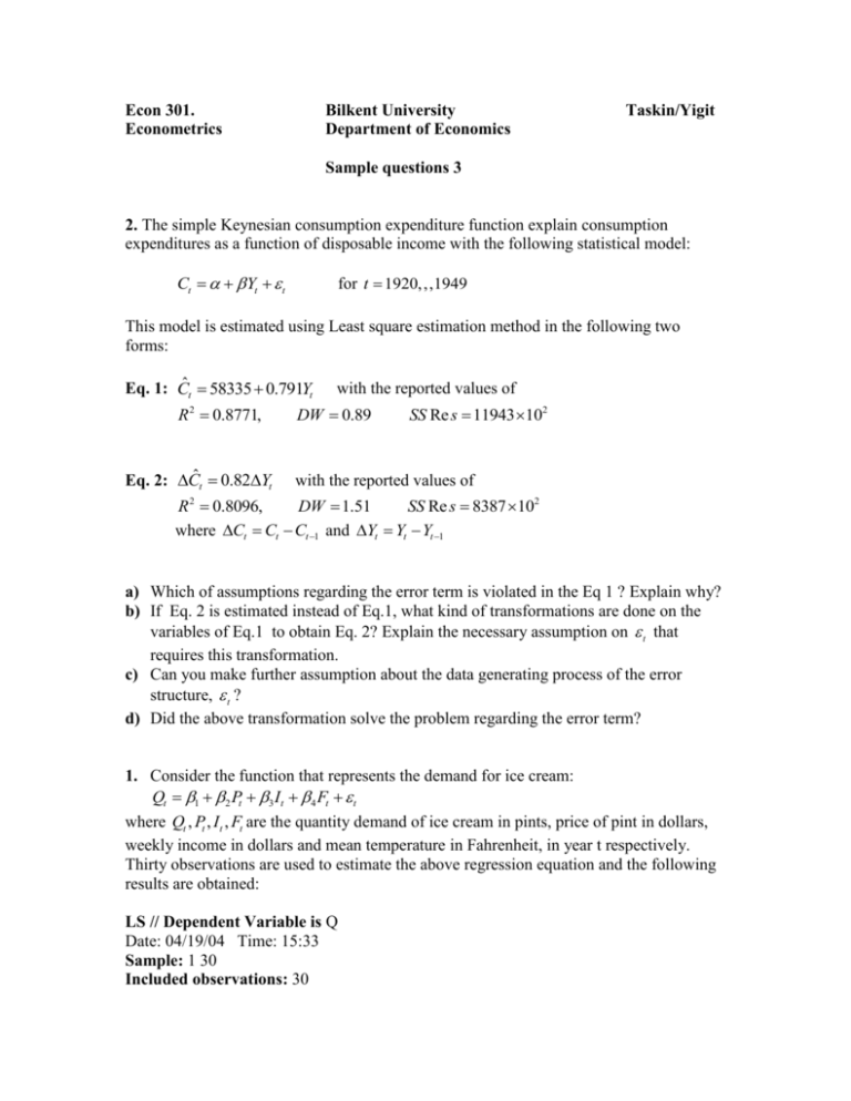
Econ 301.
Econometrics
Bilkent University
Department of Economics
Taskin/Yigit
Sample questions 3
2. The simple Keynesian consumption expenditure function explain consumption
expenditures as a function of disposable income with the following statistical model:
Ct     Yt   t
for t  1920,,,1949
This model is estimated using Least square estimation method in the following two
forms:
Eq. 1: Cˆt  58335  0.791Yt
R 2  0.8771,
Eq. 2: Cˆt  0.82Yt
with the reported values of
DW  0.89
SS Re s  11943 102
with the reported values of
R  0.8096,
DW  1.51
SS Re s  8387 102
where Ct  Ct  Ct 1 and Yt  Yt  Yt 1
2
a) Which of assumptions regarding the error term is violated in the Eq 1 ? Explain why?
b) If Eq. 2 is estimated instead of Eq.1, what kind of transformations are done on the
variables of Eq.1 to obtain Eq. 2? Explain the necessary assumption on  t that
requires this transformation.
c) Can you make further assumption about the data generating process of the error
structure,  t ?
d) Did the above transformation solve the problem regarding the error term?
1. Consider the function that represents the demand for ice cream:
Qt  1  2 Pt  3 It  4 Ft   t
where Qt , Pt , It , Ft are the quantity demand of ice cream in pints, price of pint in dollars,
weekly income in dollars and mean temperature in Fahrenheit, in year t respectively.
Thirty observations are used to estimate the above regression equation and the following
results are obtained:
LS // Dependent Variable is Q
Date: 04/19/04 Time: 15:33
Sample: 1 30
Included observations: 30
Variable
Coefficient
C
P
I
F
0.197315
-1.044414
0.003308
0.003458
R-squared
Adjusted R-squared
S.E. of regression
Sum squared resid
Log likelihood
Durbin-Watson stat
Std. Error
t-Statistic
0.270216
0.834357
0.001171
0.000446
0.718994
0.686570
0.036833
0.035273
58.61944
1.021170
Prob.
0.730212
-1.251759
2.823722
7.762213
Mean dependent var
S.D. dependent var
Akaike info criterion
Schwarz criterion
F-statistic
Prob(F-statistic)
0.4718
0.2218
0.0090
0.0000
0.359433
0.065791
-6.479173
-6.292346
22.17489
0.000000
a) Do all the coefficients have expected signs? Explain by comparing the expected sign
and the estimated sign.
b) Are all the coefficients significantly different from zero? Conduct formal tests to
decide.
c) Write the statistical equation that will describe the error structure if you assume first
order autoregressive error structure (AR(1)).
d) Test for the first order autoregressive error structure. State the null hypothesis of the
test, the formula of the test and your conclusion and interpretation.
e) Suppose you use OLS to estimate the model, Are your estimates (i) biased, (ii)
inefficient (iii) consistent? What are the properties of the reported standard errors of
the i ' s .
4. Suppose that the following equation represents the power demand in mining
production, where
POWt is the power use, PROt is the mining production, t is time trend:
ln( POWt )  1   2t  3t 2   4 ln( PROt )   t
The estimated equation is as follows:
ˆ )  4.260  0.006t  0.001t 2  0.086ln( PRO )
ln( POW
t
t
R 2  0.80
t-stat
and
SSR  0.203 DW  0.200
(32.60) (0.30)
(-0.26)
(3.01)
T  110
ˆ )  4.227  0.006t  0.001t 2  0.094 ln( PRO )  0.980 e -0.072 e
ln( POW
t
t
t 1
t 2
t-stat
R  0.82
2
(68.05) (0.26)
T  108
SSR  0.193 DW  1.98
(-0.23)
(6.88)
(9.91)
(-0.71)
where et is the residuals obtained from the first regression estimation.
a. If the above is the estimation output, do the signs of the coefficients conform to the
expected signs.
b. Which ones are significant at 5% significance level?
c. Can you say that the errors follow an autoregressive error structure? Indicate what we
mean by the autoregressive error structure and how do we test for that? Specifically
test for
I)
AR(1) and
et   et 1  vt
II)
AR(2)
et  1et 1  2et 2  vt
What is your decision about the error term behaviour?
[The null hypothesis, the test statistic and your conclusion should be stated]
d. What is the value of estimated  ?
e. Indicate and describe necessary correction (if any) by explicitly writing out the
transformed regression variables that should be used in estimation?
5. In the following model
yt  1   2 xt  et ,
where yt is the dependent variable and xt is the non-random explanatory variable and et
is the random error that satisfies the following properties:
E (et )  0 Var (et )   e2
but Cov(et e s )  0 ,
In this model random error changes according to the following equations:
et   et 1  ut
where E (ut )  0 Var (ut )   u2 but Cov(ut u s )  0
In this model a1 is the least square estimator of the parameter  1 and a2 is the least
square estimator of the parameter  2 . This estimator a2 can be expressed as :
a2   2  
( xt  x )
et .
( xt  x ) 2
a. Show whether a2 is an unbiased estimator of  2 .
b. Do you think that a2 is the best unbiased estimator? Why? State in words.
c. What is the Var (a2 ) ? Derive.
 u2
[Furthermore Var (et )   
and
1  2
2
e
Cov(et et  k )   e2  k ,
( xt  x )
]
( xt  x ) 2
6. Consider the function that represents the demand for ice cream:
Qt  1  2 Pt  3 It   4 Ft  et
it will be easier if you call wt 
where Qt , Pt , It , Ft are the quantity demand of ice cream in pints, price of pint in dollars,
weekly income in dollars and mean temperature in Fahrenheit, in year t respectively.
Thirty observations are used to estimate the above regression equation and the following
results are obtained:
LS // Dependent Variable is Q
Date: 04/19/04 Time: 15:33
Sample: 1 30
Included observations: 30
Variable
Coefficient
C
P
I
F
0.197315
-1.044414
0.003308
0.003458
R-squared
Adjusted R-squared
S.E. of regression
Sum squared resid
Log likelihood
Durbin-Watson stat
Std. Error
0.718994
0.686570
0.036833
0.035273
58.61944
1.021170
t-Statistic
0.270216
0.834357
0.001171
0.000446
Prob.
0.730212
-1.251759
2.823722
7.762213
Mean dependent var
S.D. dependent var
Akaike info criterion
Schwarz criterion
F-statistic
Prob(F-statistic)
0.4718
0.2218
0.0090
0.0000
0.359433
0.065791
-6.479173
-6.292346
22.17489
0.000000
f) Do all the coefficients have expected signs? Are all the coefficients significantly
different from zero?
g) Write the statistical equation that will describe the error structure if you assume first
order autoregressive error structure (AR(1)).
h) Test for the first order autoregressive error structure. State the null hypothesis of the
test and the result.
i) Suppose you use OLS to estimate the model, are your estimates (i) biased, (ii)
inefficient?
j) If the estimation of the following regression et   et 1  t where the error term have
the properties E (t )  0, Var (t )   2 , E (t , s )  0 for t  s , produces ˆ  0.70 or
eˆt  0.70eˆt 1
illustrate the necessary correction for correcting the autocorrelation problem in a small
sample and hence adjustment for the lost observations is required.
10. For the model Yt  1   2 X t   t where  t   t 1  t , the following test statistics
that can be used to test the first order autocorrelation is:
T
DW 
 (e  e
t 1
t
t 2
)2
T
e
t 1
2
t
a. Derive and intuitively explain the relationship between DW and  .
b. What are the range of values DW and  , and their relationship?
c. If the estimated value of DW = 1.13 with T=30, what will be your decision about the
presence of the autocorrelation problem (Write out the null and the alternative
hypothesis).
d. Compute the estimated value of  implied by the DW statistic.
e. If you find that there is autocorrelation problem how will you correct it? Write out a
hypothetical dependent and independent variable matrix that includes the correction
necessary for Generalized Least Square estimation.
11. In the following model
Yt  1   2 xt   t ,
where Yt is the dependent variable and X t is the non-random explanatory variable and  t
is the random error that satisfies the following properties:
E ( t )  0 Var ( t )   2
but Cov( t  s )  0 ,
In this model random error changes according to the following equations:
 t   t 1  t
where E ( t )  0 Var ( t )   u2 but Cov( t s )  0
In this model 1 is the least square estimator of the parameter 1 and  2 is the least
square estimator of the parameter  2 . This estimator  2 can be expressed as:
2  2  
( Xt  X )
t .
( X t  X )2
d. Show whether  2 is an unbiased estimator of  2 .
e. Do you think that  2 is the best unbiased estimator? Why? State in words.
f. What is the Var (2 ) ? Derive.
2
[Furthermore Var ( t )    
and
1  2
2
[Hint: it will be easier if you call wt 
Cov( t  t k )   2  k ] ,
( Xt  X )
]
( X t  X )2
12. For a sample of 570 respondents from the U.S. National Longitudinal Survey of
Youth, a researcher has data on Y, hourly earnings in 1994, measured in dollars, S, years
of schooling, measured as highest grade completed, and the highest educational
qualification obtained: no qualification (high school drop-out), high school diploma,
associate of arts degree (awarded by two-year colleges), and bachelor of arts degree
(awarded by four-year colleges). He defines dummy variables EDUCDO, EDUCHSD,
and EDUCBA, and EDUCBA corresponding to these four categories. He regresses the
logarithm of Y on:
i. S alone
ii. EDUCDO, EDUCAA, and EDUCBA
iii. S, EDUCDO, EDUCAA, and EDUCBA
The results are presented in the table below.
(1)
0.079
S
(2)
(3)
-0.173
(0.075)
0.040
(0.019)
-0.055
(0.094)
EDUCDO
(0.008)
-
EDUCAA
-
0.129
(0.074)
0.065
(0.080)
EDUCBA
-
0.420
(0.047)
0.246
(0.095)
1.359
(0.113)
2.321
(0.027)
1.824
(0.236)
R2
0.141
0.145
0.152
RSS
132.12
131.48
130.44
Constant
Standard errors in brackets, RSS = Residual Sum of Squares
a) Discuss whether it is possible to give an interpretation of the constant in model (1).
b) Provide an interpretation of the coefficients of the dummy variables in model (2).
c) Discuss whether it is possible to give an interpretation of the constant in model (2).
d) Perform a test of the joint explanatory power of the dummy variables in model (3),
explaining how the result of the test should be interpreted.
e) At a seminar someone says that the researcher ought to have used drop-outs as the
omitted category because they were the lowest educational category. How should the
researcher reply to this?
h) At the seminar the researcher says that the coefficients of EDUCAA and EDUCBA
were lower for males than for females when he fitted model (2) for males and females
separately. He has not tested whether they are significantly different however. Explain
how you would conduct such an exercise, writing your model as well.
13. Do question 9.3 from your book.