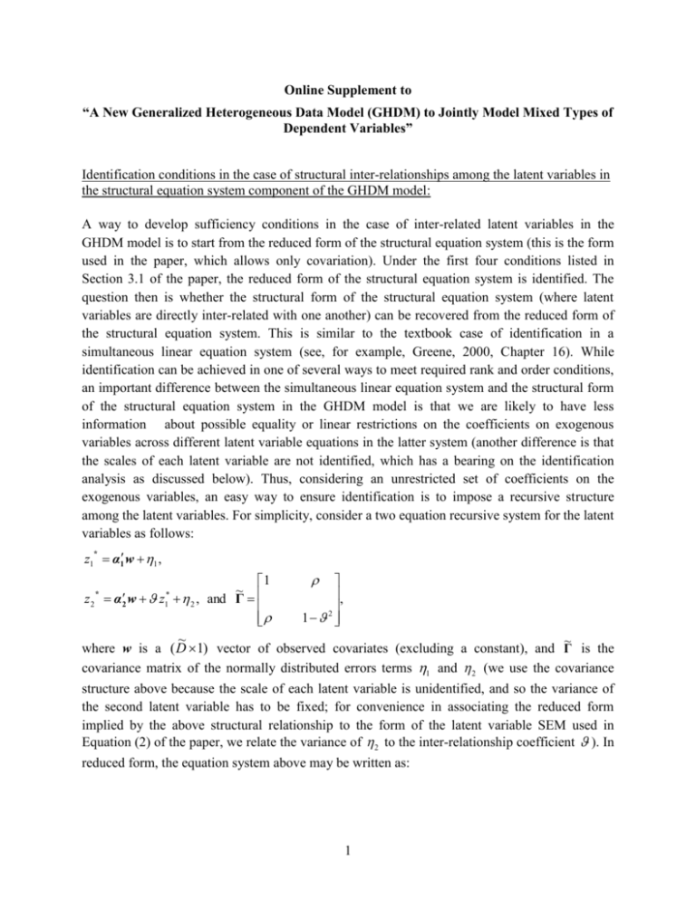
Online Supplement to
“A New Generalized Heterogeneous Data Model (GHDM) to Jointly Model Mixed Types of
Dependent Variables”
Identification conditions in the case of structural inter-relationships among the latent variables in
the structural equation system component of the GHDM model:
A way to develop sufficiency conditions in the case of inter-related latent variables in the
GHDM model is to start from the reduced form of the structural equation system (this is the form
used in the paper, which allows only covariation). Under the first four conditions listed in
Section 3.1 of the paper, the reduced form of the structural equation system is identified. The
question then is whether the structural form of the structural equation system (where latent
variables are directly inter-related with one another) can be recovered from the reduced form of
the structural equation system. This is similar to the textbook case of identification in a
simultaneous linear equation system (see, for example, Greene, 2000, Chapter 16). While
identification can be achieved in one of several ways to meet required rank and order conditions,
an important difference between the simultaneous linear equation system and the structural form
of the structural equation system in the GHDM model is that we are likely to have less
information about possible equality or linear restrictions on the coefficients on exogenous
variables across different latent variable equations in the latter system (another difference is that
the scales of each latent variable are not identified, which has a bearing on the identification
analysis as discussed below). Thus, considering an unrestricted set of coefficients on the
exogenous variables, an easy way to ensure identification is to impose a recursive structure
among the latent variables. For simplicity, consider a two equation recursive system for the latent
variables as follows:
z1  α1 w  1 ,
*
z2
*
1
~ 
 α 2 w   z   2 , and Γ 

 
*
1


,

1   2 
~
~
where w is a ( D  1) vector of observed covariates (excluding a constant), and Γ is the
covariance matrix of the normally distributed errors terms 1 and  2 (we use the covariance
structure above because the scale of each latent variable is unidentified, and so the variance of
the second latent variable has to be fixed; for convenience in associating the reduced form
implied by the above structural relationship to the form of the latent variable SEM used in
Equation (2) of the paper, we relate the variance of  2 to the inter-relationship coefficient  ). In
reduced form, the equation system above may be written as:
1
z1  α1 w  1 , 1~ N (0,1)
*
 1
*
z 2   2 w  ~2 ,  2  α 2   α1 , ~2   1   2 , and Γ  cor (1 ,~2 )  
  
 
.
1 
In the above system, what is identified based on the first four conditions in Section 3.1 of the
paper are the vectors α1 ,  2 , and the combined correlation coefficient ~     . So, at issue is
whether one can identify the vector α 2 ,  , and  from the estimates of the vector
 2  α2   α1 , scalar ~     , and the vector α1 . In general, there will be an identification
~
problem because, given α1 , we have ( D  1) equations (for the vector  2 and scalar ~ ), but
~
~
( D  2) unknowns ( D elements of vector α 2 ,  , and  ).
The situation can be resolved in one of two ways: Assume zero covariance between the error
terms 1 and  2 , in which case  = 0, the estimate of  is obtained directly from the estimate of
~ as   ~, and the elements of the vector α 2 are obtained from the elements of the vector  2
as α2   2   α1 . If one adopts this approach, the inter-relationship coefficient should be
maintained in the model even if it is statistically insignificant, because this is the only way that a
correlation is maintained in the reduced form matrix Γ (which is needed for identification in the
context of the first four conditions set forth in Section 3.1). In the more general case, each
downstream latent variable should be related to at least one upstream latent variable in the
recursive structure.
The second way to achieve identification is to allow covariance in the error terms 1 and  2 , but
*
ensure that at least one exogenous variable appearing in the z1 equation does not appear as an
*
exogenous variable in the z 2 equation. This is, of course, equivalent to imposing the constraint
that at least one element of the vector α 2 is restricted to zero. Without loss of generality, let this
be the first variable in the vector w, so that  21  0. Then, one can obtain the estimate of
   21 / 11 , the other elements of the vector α2   2   α1 , and the covariance   ~   . In a
~
more general recursive system, one can allow a general covariance matrix for Γ if each
downstream latent variable that has an upstream latent variable on the right side does not have at
least one exogenous variable appearing in the upstream latent variable equation.
Reference
Greene, W.H. (2000). Econometric Analysis, Prentice Hall, New Jersey.
2