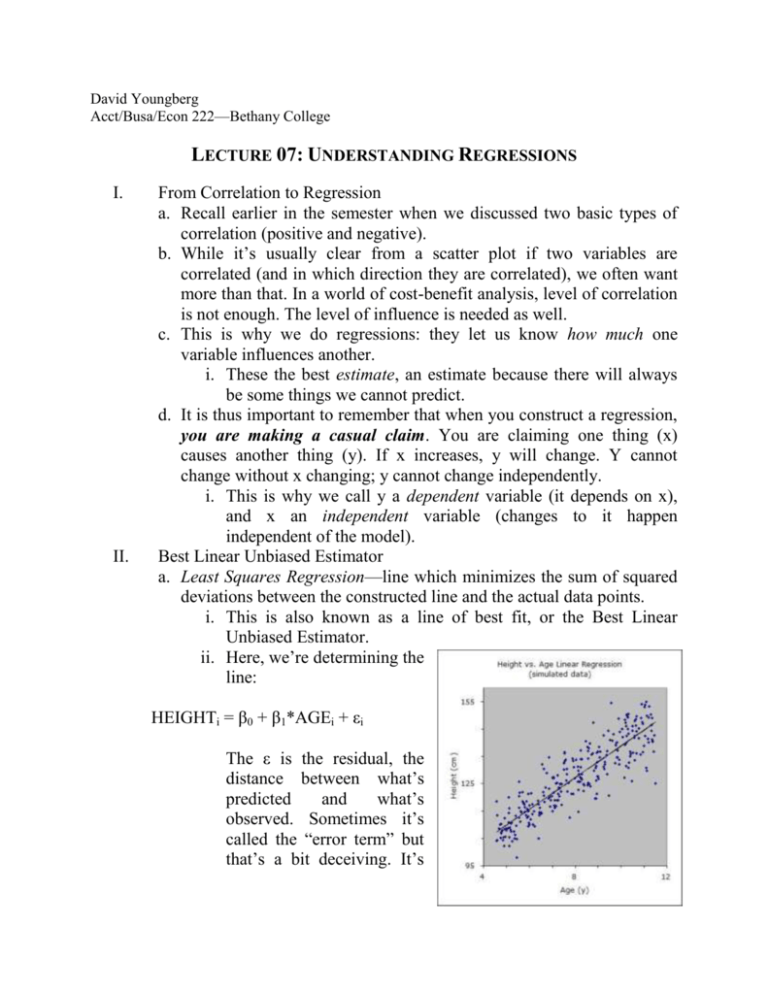
David Youngberg
Acct/Busa/Econ 222—Bethany College
LECTURE 07: UNDERSTANDING REGRESSIONS
I.
II.
From Correlation to Regression
a. Recall earlier in the semester when we discussed two basic types of
correlation (positive and negative).
b. While it’s usually clear from a scatter plot if two variables are
correlated (and in which direction they are correlated), we often want
more than that. In a world of cost-benefit analysis, level of correlation
is not enough. The level of influence is needed as well.
c. This is why we do regressions: they let us know how much one
variable influences another.
i. These the best estimate, an estimate because there will always
be some things we cannot predict.
d. It is thus important to remember that when you construct a regression,
you are making a casual claim. You are claiming one thing (x)
causes another thing (y). If x increases, y will change. Y cannot
change without x changing; y cannot change independently.
i. This is why we call y a dependent variable (it depends on x),
and x an independent variable (changes to it happen
independent of the model).
Best Linear Unbiased Estimator
a. Least Squares Regression—line which minimizes the sum of squared
deviations between the constructed line and the actual data points.
i. This is also known as a line of best fit, or the Best Linear
Unbiased Estimator.
ii. Here, we’re determining the
line:
HEIGHTi = β0 + β1*AGEi + εi
The ε is the residual, the
distance between what’s
predicted
and
what’s
observed. Sometimes it’s
called the “error term” but
that’s a bit deceiving. It’s
III.
IV.
not suggesting anyone did anything wrong.
iii. This line is determined by minimizing the sum of the squared
distance between the line and a data point.
iv. Note it’s not a perfect fit. That’s because other factors influence
height besides age. What others factors could play a role?
b. β1 is the slope of the line. It tells us how much age matters to height.
Suppose the line is HEIGHTi = 80 + 5.6 AGEi + εi.
i. We can estimate that someone who is 8 years old is probably 80
+ 5.6(8) = 124.8 cm tall. For every year someone ages, they get
5.6 cm taller.
ii. If the average height of our sample is 130 cm, we can also say
that for every year someone ages, they get (5.6/130 = 0.043)
4.3% taller.1
iii. These summary sentences are what I referred to earlier as your
“punchline.”
c. For each variable in the regression (and it’s possible to have many,
which we will discuss later), Excel will tell you the following:
i. Coefficient—this is the beta-value for the variable; the slope.
ii. t-statistic—ratio of the estimated coefficient to the standard
error of the estimated coefficient (coefficient divided by error).
iii. Confidence interval—describes the range that the true value of
the parameter could fall with a certain level of certainty (usually
95%). It outputs this result twice; I have no idea why.
iv. p-value—tells you the threshold of significance you achieve for
a particular t-statistic. (Remember critical t values changes
based on degrees of freedom.) If the p-value is below 0.05, it’s
significant to the 5% (95% confidence) level. If below 0.01, it’s
significant to the 1% level, etc.
iClicker
Homoscedasticity
a. Linear regressions have several assumptions which we will be
exploring. A notable one is homoscedasticity—the variance (or the
deviation) from the regression line is the same, regardless the value of
the independent variable(s).
b. When we lack homoscedasticity we have heteroscedasticity, or the
variance is not the same for all values of our independent variable.
This latter method is helpful when your dependent variable isn’t something intuitive, such as a measure of the
freedom of the press. Similarly, if your independent variable isn’t something obvious, you’ll want to use percents as
well. “For every 1% freer countries become [1% being 1% of the average level of freedom for your sample], GDP
per person increases by $500.”
1
i. Heteroscedasticity can show up in different ways. Here we see
how variance increases as income increases. But if variance
decreased, or increased and then decreased, or decreased and
then increased, etc. we’d still have a problem.
V.
c. Why should we care? Heteroscedasticity biases our error which means
our t-statistic is higher (or lower) than it should be.
i. In practice, it is not much higher so if you’re significant to the
1% level, you’re probably fine.
ii. But if your values are barely significant (close to 5%), then you
have a problem. If you’d adjust for heteroscedasticity, your
significant result might cease being so!
d. A potential correction to heteroscedasticity is a poor model. If you’re
not using a logarithmic function, try transforming your data so you do.
i. If this doesn’t work, don’t worry about it. There are better
corrections but it is beyond the scope of this class (and Excel
can’t handle it).
e. The simplest way to detect heteroscedasticity is to make a scatter plot
and add a regression line. This visualization test is intuitive, but not
precise.
f. In lab we will do what’s called the Breusch-Pagan Test for a better
approximation.
Analysis of Variance
a. This material will be covered in the lab after the exam. We cover it
now because it is also a good set up for the lecture two weeks from
today.
b. We’ve previously used the t-test to compare the means of two
samples. But sometimes we want to compare the variance (is one
sample more consistent than another). Other times we want to
compare multiple samples at the same time.
i. Why don’t we just run the t-test several times, once for each
pair of samples? Because (A) that gets really time consuming
and (B) the Central Limit Theorem. Remember CLT states that
sample means will approximate a normal distribution. Any two
samples might be different based on chance (say, two on
opposite sides of the distribution). You’ll commit Type I Error.
ii. Example: You’re curious if a particular type of occupation likes
a new product more than others. You might compare just
teachers and factory workers. Then you add writers, and then
police officers, and then musicians, etc. The more points of
comparison you have, the more likely a difference will be
statistically significant by chance. Type I Error.
iii. Example: You’re curious if a new soap is better than a current
brand. So you ask the treatment and control a battery to assess
based on several metrics: smell; color; shape; feeling of
cleanliness right after use; cleanliness an hour after use; six
hours after use; quickness to lather; etc. The more metrics you
add, the more likely you are to conclude its different based
solely on chance. Type I Error.
c. We can correct this problem with Analysis of Variance (ANOVA)—a
method for testing if the means of several groups are equal; a
generalized t-test.
d. ANOVA is determined by the F-ratio, or
𝐹=
𝑣𝑎𝑟𝑖𝑎𝑛𝑐𝑒 𝑏𝑒𝑡𝑤𝑒𝑒𝑛 𝑡ℎ𝑒 𝑑𝑖𝑓𝑓𝑒𝑟𝑒𝑛𝑡 𝑔𝑟𝑜𝑢𝑝𝑠
𝑣𝑎𝑟𝑖𝑎𝑛𝑐𝑒 𝑤𝑖𝑡ℎ𝑖𝑛 𝑡ℎ𝑒 𝑑𝑖𝑓𝑓𝑒𝑟𝑒𝑛𝑡 𝑔𝑟𝑜𝑢𝑝𝑠
i. Since Excel will be calculating the F-ratio for us, and it’s a long
calculation, I won’t go into it here.
e. ANOVA relies of the F-distribution, which is really a family of
distributions depending on the degrees of freedom in the numerator
and the degrees of freedom in the denominator.
i. The distribution is positively skewed and ranges from zero to
infinity.
f. There are several ways to use ANOVA:
i. Two-sample for variance—check to see if two samples have the
same variance.
ii. Single factor—check if samples are different across groups. For
example, “Do these different routes from A to B take different
amounts of time?”
iii. Two factor—check if samples are different across groups and
within groups. This calculation is different from the single
factor even for the differences across groups (which both
return). For example, “Do these different routes from A to B
take different amounts of time and—since several different
drivers drove each route—does the average time between
drivers differ?”
iv. In other words, two factor ANOVA checks if the average is
different between one type of group (here, the driver)…
Driver
Adams
Brockman
Callahan
Davies
Edgeworth
Travel Time from Starbrick to Warren
U.S. 6
West End
Hickory
Rte. 59
18
17
21
22
16
23
23
22
21
21
26
22
23
22
29
25
25
24
28
28
v. …and then uses that information to check if the average is
different between another type of group (here, the route).
Driver
Adams
Brockman
Callahan
Davies
Edgeworth
VI.
Travel Time from Starbrick to Warren
U.S. 6
West End
Hickory
Rte. 59
18
17
21
22
16
23
23
22
21
21
26
22
23
22
29
25
25
24
28
28
vi. It’s crucial to understand that the two-way ANOVA assessment
will get a different result than the one-way ANOVA, even for
the same treatment. If we did one-way ANOVA for routes,
we’d find the routes take the same time. A two-way ANOVA
would find that the route does matter.
vii. Which one to use depends on if your secondary treatment factor
(here, the driver) is important to consider. Which one to use is
often a judgment call.
iClicker
LAB SECTION (PRE EXAM)
VII. Chapter 13
a. You must delete any observations which lacks data for variable. If you
do not, you’ll get an error saying “Regression - LNST() function
returns error. Please check input ranges again.”
i. The easiest way to eliminate such observations is to use the sort
function. Sorting the data by each variable will put all the
observations with a missing value for that variable in the same
place.
VIII. Breusch-Pagan Test
a. Step 1—run a regression in Excel, making sure to select the
“Residuals” option. (Not “Standardized Residuals.”) Let’s assume it
appears in C1:C15.
b. Step 2—create a new column, call it Res2, and square all the residuals
(=C1^2, =C2^2 in the next row, etc).
c. Step 3—divide the sum of the residuals (you can see that in the output
for the regression) by your total number of observations.
d. Step 4—create a new variable, let’s call it “bp” which is the squared
residual divided by the value you got in Step 3 (=Res2/(RSS/n))
e. Step 5—note in the residual output is a “Predicted Y” column. You
will now run a regression with “Predicted Y” as the independent and
“bp” as the dependent.
f. Step 6—divide the ESS (regression sum of squares) by two and use
the result in a chi test. Type =CHIDIST(x,1), where x is half of ESS.
(Your degrees of freedom will always be one.) If you get more than
0.05, you have homoscedasticity.
IX. Homework
a. Chapter 13: 1-2
b. Using the data for the class, regress so GDP/capita predicts the
Deaths/1000. Then use the Breusch-Pagan Test to test for
heteroscedasticity. Interpret the results. (I just need the final
regression results and the result from the Chi distribution.)
LAB SECTION (POST EXAM)
X.
XI.
Chapter 12
Homework
a. Chapter 12: 1, 3-6