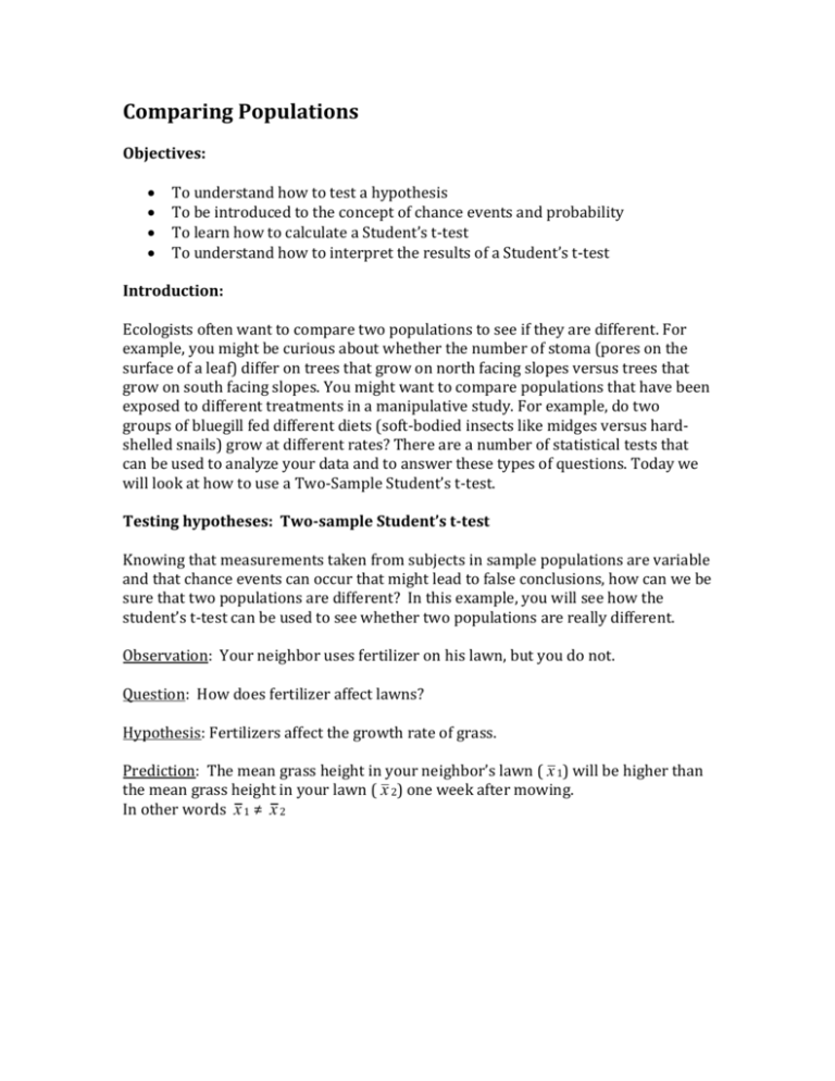
Comparing Populations
Objectives:




To understand how to test a hypothesis
To be introduced to the concept of chance events and probability
To learn how to calculate a Student’s t-test
To understand how to interpret the results of a Student’s t-test
Introduction:
Ecologists often want to compare two populations to see if they are different. For
example, you might be curious about whether the number of stoma (pores on the
surface of a leaf) differ on trees that grow on north facing slopes versus trees that
grow on south facing slopes. You might want to compare populations that have been
exposed to different treatments in a manipulative study. For example, do two
groups of bluegill fed different diets (soft-bodied insects like midges versus hardshelled snails) grow at different rates? There are a number of statistical tests that
can be used to analyze your data and to answer these types of questions. Today we
will look at how to use a Two-Sample Student’s t-test.
Testing hypotheses: Two-sample Student’s t-test
Knowing that measurements taken from subjects in sample populations are variable
and that chance events can occur that might lead to false conclusions, how can we be
sure that two populations are different? In this example, you will see how the
student’s t-test can be used to see whether two populations are really different.
Observation: Your neighbor uses fertilizer on his lawn, but you do not.
Question: How does fertilizer affect lawns?
Hypothesis: Fertilizers affect the growth rate of grass.
Prediction: The mean grass height in your neighbor’s lawn ( x 1) will be higher than
the mean grass height in your lawn ( x 2) one week after mowing.
In other words x 1 ≠ x 2
Table 1. Grass heights resulting from different fertilizer treatments.
Grass Height (cm)
No Fertilizer Treatment
Grass Height (cm)
Fertilizer Treatment
3.86
4.76
3.30
3.52
3.88
4.32
5.86
5.08
4.76
4.38
Average = 4.37
4.47
5.95
4.98
7.22
3.95
5.24
6.25
4.58
6.05
5.88
Average = 5.46
Testing hypotheses: Two-Sample Student’s t-test, cont.
Just from looking at the data you would probably have difficulty saying with any
certainty whether your neighbor’s grass grows at a different rate than yours. Based
on the means of each sample set ( x 1 = 4.37cm and x 2 = 5.46cm) you might conclude
that the mean grass heights in the two lawns are different, but the grass heights are
relatively variable. What if you had sampled a different set of 25 blades from each
lawn? Would the means still be different? Student’s t-test can be used to account for
variability, reducing the likelihood of falsely concluding that the populations are
different and providing a more objective way of determining whether a difference
does exist.
It is most appropriate to use the two –sample student’s t-test to analyze continuous
data (data can be measured with a ruler and can be broken into smaller parts and
still remain meaningful, i.e. time, money, temperature, size). If you were comparing
count data (discrete and non continuous data, i.e. number of birds at each site), you
would use the Chi Square goodness of fit test.
To run the t-test we need to calculate a t-value referred to as tcalc fo our data. The tcalc
for the lawn data is calculated below:
t calc =
s
2
1
=
s
x1 - x 2
1.09
4.37 - 5.46
= 2.744
=
=
æ 0.59984 ö æ 0.97734 ö 0.397186
æ s21 ö æ s2 2 ö
÷
÷ +ç
ç
ç ÷ -ç ÷
è 10 ø è 10 ø
è n1 ø è n 2 ø
å( x
=
1
- x1 )
2
n1 -1
(3.86 - 4.37) 2 + (4.76 - 4.37) 2 + ... + (4.38 - 4.37) 2
= 0.59984
10 -1
2
2
å( x
=
2
- x2 )
2
n 2 -1
(4.47 - 5.46) 2 + (5.95 - 5.46) 2 + ... + (5.88 - 5.46) 2
= 0.977734
=
10 -1
df = n1 + n 2 - 2 = 10 +10 - 2 = 18
Testing hypotheses: Two-Sample Student’s
t-test
0.1
0.05
0.025
df
1
3.08
6.31
12.71
Now that the tcalc has been calculated, how is it 2
1.89
2.92
4.31
used?
3
1.64
2.35
3.18
4
1.53
2.13
2.78
To reach a conclusion, we need to use a table
5
1.48
1.02
2.57
and find our tcalc value in there. The table is
6
1.44
1.94
2.45
organized with rows being the degrees of
7
1.42
1.90
2.36
freedom (df). To use the correct row, you need 8
1.40
1.86
2.31
to calculate your own df. The degrees of freedom 9
1.38
1.83
2.26
for the student’s t-test are calculated from your 10 1.37
1.81
2.23
sample sizes (N1 and N2) as
15 1.34
1.75
2.13
18 1.33
1.73
2.10
df = N1+N2 -2
20 1.33
1.73
2.09
30 1.31
1.70
2.04
Once you’ve located the row corresponding to
40
1.30
1.68
2.02
your df, find one this row the value the closest to
1.67
2.00
your tcalc. Then look at the head of the column, 60 1.30
120 1.29
1.66
1.98
and find what value is written on top of that
column. This value is a probability (p), therefore referred to as a p-value.
0.01
31.82
6.97
4.54
3.75
3.37
3.14
3.00
2.90
2.82
2.76
2.60
2.55
2.53
2.46
2.42
2.39
2.36
This p-value corresponds to the probability that our conclusion is false (i.e., the
probability we have a false-positive situation or a “fluke”). This p-value is what is
mostly reported in scientific studies and what is used to evaluate how reliable
conclusions are. Having a p-value = 0.05 menas that we have a 5% chance that our
conclusion (that the two populations are different) is actually false. This 0.05 is the
threshold level considered an appropriate margin of errors for most scientific
studies. The smaller the probability, or p-value, the more confident you are that you
do not have a false-positive conclusion.
Therefore, this p-value enables you to conclude whether you reject or not your
hypothesis.
If p≤ 0.05, then we don’t reject our biological hypothesis (in this case we
do not reject the hypothesis that fertilizer affects the growth rate of grass because
we see a statistically positive effect of fertilizer on grass height). This means that
there is less than 5% of chance that any difference we are observing in the two
populations is random. For this t-test, this means that the two populations
samples are statistically different from one another.
If p>0.05, then we reject our biological hypothesis (in this case we reject the
hypothesis that fertilizer affects the growth rate of grass because we do not see a
statistically positive effect of fertilizer on grass height). This means that there is
much variation in our sample and it is likely that differences observed between two
populations are caused by chance. For this t-test, this means that the two
populations sampled are NOT statistically different from one another.
Another way to determine if your data are significantly different from the statistical
null hypothesis (or no significant difference between the two sample populations) is
to look at the t value that you calculated. If the calculated t value is greater than the
value given by the Student’s t distribution for the proper significance level and
degrees of freedom, also called the critical value, then the statistical null hypothesis
(no significant difference between the two samples) can be rejected and we can
conclude that the means of the two populations are significantly different. If the
calculated t value is less than the critical t value, then the data fail to reject the null
hypothesis and you can conclude that there is no statistical difference between the
means of the two populations.
Let’s go through our example:
We have found previously that tcalc=2.744 with df=18. On that row of df of 18, the
closest to our tcalc is located in the column α = 0.01.
So this means that our p-value = 0.01. Because this number is below 0.05, we can
rely on our conclusion quite well. The probability that the conclusion we obtained is
false is extremely small (1%). Therefore, we can conclude that the two lawns were
different, meaning that our hypothesis is supported by our study, and that fertilizers
have indeed a positive effect on the height of grass.
Conclusions:
Statistics:
Decision:
Statistical interpretation:
Biological Interpretation:
tcalc = 2.744, p=0.01
Do not reject the hypothesis
The two lawns are statistically different from
one another.
The use of fertilizer causes grass in the two
lawns to grow at different rates.
Activity
Together as a group, come up with a testable question that would allow you to
compare two populations (based on sex, hair color, diet, year in college, etc.) and to
collect data on a measurable trait (height, time to complete a task, finger length,
etc.). Clearly outline your question, hypothesis, and prediction, make sure that
everyone will measure the trait in the same way and then go and collect as much
data as you can in one hour. When you return, we will analyze the data, graph the
data and make a conclusion based on what was found.
At the end of lab hand in your Question, Hypothesis, Prediction, Results, Graph and
Conclusion.